Hagan’s adjusters [Hag02] improve the pricing of financial products, even with the simplest models, by transferring model risk to some hedging instruments.
This article is the web version of the paper Smart Adjusters. It presents an improvement of this standard approach for the particular equity/FX structured product case, that can be applied generically and that is much faster, as slowness is a major drawback of the standard approach. Our methodology is close to the control variates variance reduction method. This approach can therefore also be used to provide an efficient and generic choice of control variables. We provide numerical results on a traded structured product portfolio that validate our method of adjusting the price and reducing the Monte Carlo variance.
The adjusters method has been introduced in [Hag02] while a similar approach has been presented in [Kar05]. It seems
to be rarely used through, as practitioners are faced with its computational cost. We nevertheless strongly believe in
this approach, as it allows to lower the pricing error made due to a bad model choice or calibration and the lack of
precision inherent to numerical methods. In this paper, we therefore show a way to 1) reduce the computational cost
of the original approach and 2) make it generic and applicable to equity/FX structured products.
1. Introduction
We start by introducing the context and presenting the standard approach. We consider a financial product Π that pays
nt cash flows at respective dates $t_i$, for $i = 1..n_t$. We assume that the cash flow amount may depend on the realized trajectories of $n_S$ underlyings up to $t_i$:
$\Phi_i(S_j(t \leq t_i)_{j = 1..n_S})$. Let $Price(m)$ be the price operator for model $m$.
The price of $\Pi$ for model $m$ is therefore $Price(m)\Pi$. We make the usual assumption of linearity of the pricing operator:
the price of the sum of two payoffs is equal to the sum of their individual prices.
The adjusters method aims at considering the pricing of a product by decomposing it into a suitably chosen hedging
portfolio and a (hopefully “small” or at least easy to price) residual payoff.
Let the approximate hedging portfolio contain $n_H$ instruments $(H_i)_{i \in [1; n_H]}$, each with a weight $\alpha_i$:
By linearity of the pricing operator, the model price of $\Pi$ under $m$ can be written:
\[ Price(m)\Pi = (m)\left(\Pi - \sum_{i=1}^{n_H} \alpha_iH_i\right) + \sum_{i=1}^{n_H} \alpha_iPrice(m)H_i \]We suggest to minimize the model risk by using market prices instead of model prices for the hedging portfolio prices. We therefore introduce the new operator $Price^{adj}$ defined by:
$$ \begin{align} \label{eq:adj_price} Price^{adj}(m, \alpha, H)\Pi = Price(m)\left(\Pi - \sum_{i=1}^{n_H} \alpha_i H_i\right) + \sum_{i=1}^{n_H} \alpha_i Price^{mkt}(H_i) \end{align} $$where $Price^{mkt}(H)$ is the observed market price of $H$.
Note that the adjusted model risk is only supported by the first term of previous expression. For a perfectly hedged product ($\Pi = \sum_i \alpha_i H_i$), After having briefly described the principle of the adjuster method, we describe in the next section the usual selection rule for the hedging instruments and their associated weights. In a later section we will present how we enhance this standard method to fulfill our goals and be compatible with our constraints.
2. Choice of the weights
his article, Hagan applies this method to interest rate products [Hag02]. The hedging instruments are “the natural hedging instruments” (page 56). Thus, he focuses on the weights determination but not on the hedging instruments selection itself. He computes these weights in the following way.
Let $(I_i)_{i \in [1; n_I]}$ be the family of calibration instruments (caplets or swaptions). Let $\sigma_i$ be the volatility associated to $I_i$, and let
$m(\sigma)$ be a model calibrated on $\sigma = (\sigma_1, \sigma_2, ... ,\sigma_{n_I})$.
The risk that is migrated in the Hagan’s article is the Vega risk. He therefore chooses the weights which minimize the Vega of the hedged portfolio.
Let $\alpha^*$ be the chosen weights on the model $m$, given the hedging instruments $H$. $\alpha^*$ verifies:
\[ \alpha^* \in argmin_\alpha\left\{\sum_{i=1}^{n_S} \left(\frac{\partial Price \big(m(\sigma)\big)\left(\Pi - \sum_{j=1}^{n_H} \alpha_j H_j\right)}{\partial \sigma_i}\right)^2\right\} \]This optimization problem can be written as a standard quadratic optimization problem.
We set
$$ \begin{align*} M_{ij} &:= \frac{\partial Price\big(m(\sigma)\big) (H_i)}{\partial \sigma_j}\\ U_i &:= \frac{\partial Price\big(m(\sigma)\big) (\Pi)}{\partial \sigma_i} \end{align*} $$The problem can be written:
\[ \alpha^* \in argmin_\alpha\left\{ (U - M\alpha)^T(U - M\alpha) \right\} \]Depending on the number of hedging instruments relatively to the number of calibration instruments, this problem has either one or an infinite number of solutions. We note that it is important to compute a solution when there are more calibration instruments than hedging instruments, because it is the more frequent case in practice.
When there are more calibration instruments than hedging ones, ($n_H < n_I$), the matrix $M$ is rectangular. A solution can be found using the pseudo inverse $M^+ = (M^TM)^{-1}M$ of $M$, known to provide one solution of this least square problem:
$$ \begin{align} \label{eq:sol1} \alpha^* := M^+ U \end{align} $$When there are as many calibration instruments as hedging ones ($n_H=n_I$), the solution is:
$$ \begin{align} \label{eq:sol2} \alpha^* := M^{-1} U \end{align} $$We note that when $M$ is invertible, $M^{+} = M^{-1}$. Then, \eqref{eq:sol1} and \eqref{eq:sol2} can be rewritten $\alpha^* = M^+ U$
The adjusted price operator is then
\[ Price^{adj}\big(m(\sigma), \alpha^*, H\big) \]using $Price^{adj}$ defined in \eqref{eq:adj_price}.
3. New approach
Although previous approach is powerful for pricing, risk management and hedging, it has two major drawbacks: firstly, it requires to build a ``natural hedging portfolio''. Thus, it requires exogenous financial expertise to be used, and cannot be implemented in a generic way, whatever the input contract. Secondly, it is computationally very expensive, which makes this approach a potential candidate for risk management and hedging, but difficult to justify in a pricing only context, as competitive more powerful unadjusted models exist, that provide results of similar quality at the same or smaller computational cost. Previous approach necessitates indeed computation of a lot of vega, which is very expensive: one re-calibration and one repricing per vega, implying a total of $n_I + 1$ calibrations and pricings (total pricing time multiplied by $n_I + 1$).
Our goal is therefore to enhance the previous classical approach to make it generic, fast, and adapted to equity/FX structured product.
We suggest to achieve this goal by replacing the standard Vega minimization by a variance minimization. More precisely, we look at the variance of the sum of the cash flows capitalized at maturity. Let $X_T(m)$ be the operator that capitalizes all the flows at $T$ under model $m$:
\[ X_T(m)(\Pi) = \sum_{i=1}^{n_t} \Phi_i(\mathcal S_j(m)(t \leq t_i)_{j=1..n_S}) \frac{P(0, t_i)}{P(0, T)} \]Where $\mathcal S(m)$ is the trajectory of $S$ under the risk free probability of model $m$.
We therefore look for
\[ argmin_\alpha \left\{Var{X_T(m)\left(\Pi - \sum_{i=1}^{n_H} \alpha_i H_i\right)}\right\} \]with $T = t_{n_t}$, the maturity of the contract.
3.1 Some qualitative features
We note that minimizing the historical variance is a standard way to build a hedging portfolio. We also note that under the usual modeling assumptions,
the risk neutral probability and the historical one are equivalent, which implies that $\mathrm {Var}_\mathbb P(X) = 0 \Leftrightarrow \mathrm {Var}_Q P(X) = 0$.
As a consequence, if $\Pi$ can be perfectly statically hedged with $(H_i)$, then the solution of the new approach will be a perfect hedge.
We also remark that this approach corresponds to control variables weight finding (see for instance [Gla04]. Thus, it is much faster than the standard approach when the pricing is made using a Monte Carlo method. Furthermore, a software implementation that handles control variables for variance reduction can easily be extended to support our proposed adjusters.
3.2 Weight optimization solution
The problem that we need to solve reduces again to a quadratic optimization, as in previous section.Let
$$ \begin{align*} &\Sigma_\Pi = Var{X_T(m)\Pi}\\ &\Sigma_H \text{ the covariance matrix of } X_T(m): (\Sigma_H)_{i, j} = Cov\left(X_T(m)H_i, X_T(m)H_j\right)\\ &\Sigma_{\Pi, H} \text{ the column vector such as } (\Sigma_{\Pi, H})_i = Cov\left(X_T(m)\Pi, X_T(m)H_i\right) \end{align*} $$The variance of the hedged portfolio is:
\[ Var{X_T(m)\left(\Pi - \sum_{i=1}^{n_H}\alpha_iH_i\right)} = \Sigma_\Pi + \alpha^T\Sigma_H \alpha - 2\alpha^T\Sigma_{\Pi, H} \]So that the solution is:
$$ \begin{align} \alpha^* &= argmin_\alpha \left(\Sigma_\Pi + \alpha^T\Sigma_H \alpha - 2\alpha^T\Sigma_{\Pi, H}\right)\nonumber \\ \Rightarrow \alpha^* &= \Sigma_H^{-1}\Sigma_{\Pi, H} \end{align} $$We assumed that $\Sigma_H$ is invertible, which should often be the case in practice. However, when it is not the case one can still replace $\Sigma_H^{-1}$ with $\Sigma_H^{+}$.
We emphasize that to be efficient, this method must be used within a Monte Carlo pricing, so that the required covariances can be computed in the main pricing loop.
4. Choice of the hedging instruments
The sensible part of our approach lies in an appropriate choice of
hedging instruments $(H_i)_{i \in [1; n_H]}$, as we have to compromise
on conflicting goals and consider different kinds of constraints. We
want our method to be generic but reasonably efficient. Genericity
means in our context that the choice of hedging instruments can be
mechanized, and therefore be achieved automatically by an adequate
software implementation. We want our optimal hedging portfolio to
approximate as good as possible the financial contract $\Pi$ while
ensuring that the prices of the hedging instruments are observed on
the market and don’t need any model related evaluation. Last
observation imposes to use reasonably liquid hedging instruments, so
that their prices are significant.
A natural choice is to have one hedging instrument per underlying; one should indeed choose hedging instruments whose payoffs depends only on their associated underlying, for market liquidity reasons. Our choice could be the traded underlying itself, or a simple European listed call on the underlying.
We will indeed consider more complex hedging instruments, as we will allow the hedging instrument $(H_i)_{i \in [1; n_S]}$ to have any payoff at maturity $T$ of contract $\Pi$ that depends only on the underlying observed at maturity: $H_i = \Phi^H_i(S_i(T))$ paid at $T$.
This choice implies that $X_T(m)H_i = H_i$; moreover, the market price of $H_i$ can be ``observed’’ by interpolating its payoff by a set of options on $S_i$ of maturity $T$, using the Carr-Madan static replication approach [CM98] to get its price.
We therefore have to specify hedging payoffs $H_i = \Phi^H_i(S_i(T))$ that approximate reasonably the financial behavior of contract $\Pi$ while being computational tractable. We indeed derive the hedging instrument payoff from the financial behavior of contract $\Pi$ with respect to each individual underlying $S_i$. For hedging instrument $H_i$, we therefore associate to any realization $x = S_i(T)$ of underlying $S_i$ at date $T$ a realization of trajectories of all $(S_i)_{i \in [1; n_S]}$ such that $S_i(T) = x$ that allows us to evaluate the accumulated cashflows of $\Pi$ under this realization.
We assume that the realization of trajectories of all $(S_i)_{i \in [1; n_S]}$ essentially follow their respective forward curve; we allow however a parallel shift on one or more forward yield curves as to reach a prescribed spot value at maturity for the considered underlying $S_i$. We propose three possibilities according to this idea:
Only one underlying’s trajectory is shifted, the others remain unchanged:
$$ \begin{align} \begin{split} \label{eq:orthogonal} \Phi^H_{j_0}(s) &= \sum_{i=1}^{n_t} \Phi_i\left(\left(F_j(0, t)\right)_{t \leq t_i, j \neq j_0}, \left(F_{j_0}(0, t)e^{y t}\right)_{t \leq t_i}\right)\frac{P(0, t_i)}{P(0, T)}\\ y &= \frac{\log\left(s/F_{j_0}(0, T)\right)}{T} \end{split} \end{align} $$All underlyings move parallely:
$$ \begin{align} \begin{split} \label{eq:parallel} \Phi^H_{j_0}(s) &= \sum_{i=1}^{n_t} \Phi_i\left(\left(F_j(0, t)e^{yt}\right)_{t \leq t_i, 1 \leq j \leq n_S}\right)\frac{P(0, t_i)}{P(0, T)}\\ y &= \frac{\log\left(s/F_{j_0}(0, T)\right)}{T} \end{split} \end{align} $$The underlying moves are computed using the ``$\beta$’’:
$$ \begin{align} \begin{split} \label{eq:beta} \Phi^H_{j_0}(s) &= \sum_{i=1}^{n_t} \Phi_i\left(\left(F_j(0, t)e^{\beta_j(t) y t}\right)_{t \leq t_i, j \neq j_0}, \left(F_{j_0}(0, t)e^{y t}\right)_{t \leq t_i}\right)\frac{P(0, t_i)}{P(0, T)}\\ y &= \frac{\log\left(s/F_{j_0}(0, T)\right)}{T}\\ \beta_j(t) &= \rho_{j, j_0}\frac{\int_0^t \sigma_{j_0}(u)du}{\int_0^t \sigma_j(u)du} \end{split} \end{align} $$Where $\sigma_j$ is the instantaneous volatility that allows to match the ATM call prices on $S_j$.
Note that for products that pay a single flow depending on the observed level of a single underlying at the same date, the hedging instrument is precisely the product: the adjusted price will therefore be the market price of this product.
Another important remark is that this choice of hedging instrument is particularly suitable for structured product, as most of them play on a monotonous move of the underlyings (at least on European market), whereas some derivatives plays on ``roller-coaster’’ moves, like double knock-in barrier options for instance.
5. Refinement of the hedging instrument
The Carr-Madan static replication formula requires the computation of an integral. Thus, we necessarily make a quadrature error on the market price of the hedging instruments. Furthermore, it can be costly to compute it precisely. Then, we replace the formulas (5), (6) and (7) with a piecewise affine interpolated (and extrapolated) version:
\[ \hat H_i(s_{j - 1} \leq s \leq s_j) = H_i(s_{j-1}) + \frac{H_i(s_j)-H_i(s_{j-1})}{s_j - s_{j-1}}(s - s_{j-1}) \]For $(s_j)$, we take all the points where the payoff derivative is not continuous. If the input function is not piecewise affine, we also add some points, concentrated near high second order derivatives of the payoff (in absolute value), so that the difference between the two functions is not too high.
Thus, the weights will be a little bit different than if we used the exact functions, but the quadrature error is removed. We note that for products with a single cash flow depending on a single underlying, instead of having an exact hedging, whose price contains quadrature error, we use an approximated hedging, with a minimal $L^2$ error (ie with the lowest possible variance), which is more meaningful in financial terms. Indeed, $\bar H$ can be replicated with a finite linear combination of calls, puts and a bond, like any continuous, piecewise affine payoff:
First, we choose $s_{j_0}$. We work on $\tilde H = \hat H -\hat H(s_{j0})$ so that $\tilde H(s_{j0}) = 0$.
We search $\alpha^C, \alpha^P$ so that $\tilde H = \sum_{j = 1}^{j_0} \alpha^P_j Put(s_j) + \sum_{j = j_0}^N \alpha^C_j Call(s_j)$.
Easy computation leads to:
$$ \begin{align*} \alpha^C_{j_0} &= \frac{\tilde H (s_{j_0 + 1})}{s_{j_0+1} - s_{j_0}} \\ \forall j > j_0, \alpha^C_j &= \frac{\tilde H (s_{j + 1}) - \sum_{k=j_0}^{j-1} \alpha^C_k(s_{j+1}-s_k)}{s_{j+1} - s_j}\\ \alpha^P_{j_0} &= \frac{\tilde H (s_{j_0 - 1})}{s_{j_0} - s_{j_0 - 1}} \\ \forall j < j_0, \alpha^P_j &= \frac{\tilde H (s_{j - 1}) - \sum_{k=j + 1}^{j_0} \alpha^P_k(s_k-s_{j-1})}{s_j - s_{j-1}}\\ \end{align*} $$These weights also provide a hedge for $\hat H$, and allow to compute the market price of $\hat H$:
$$ \begin{align} \label{eq:hath} Price^{mkt} \hat H = P(0, T) \hat H (s_{j_0}) + \sum_{j = 1}^{j_0} \alpha^P_j Put^{mkt}(K=s_j, T) + \sum_{j = j_0}^N \alpha^C_j Call^{mkt}(K=s_j, T) \end{align} $$The market option prices $Put^{mkt}$ and $Call^{mkt}$ in \eqref{eq:hath} can be computed in an arbitrage free way using [AH11].
A last remark is that here, we still have an interpolation error, because we use non traded option prices in our pricing. If one wants to totally remove the interpolation risk, one can use only the traded option by using the traded option strikes for $s_j$, and using $X_{T_{mkt}}$ instead of $X_T$ where $T_{mkt}$ is the traded option maturity closest to the product one, instead of the previously proposed. Thus, it will build a minimal variance hedging portfolio using only the traded options.
5.1 Quanto payoff price approximation
The previous formula works even for quanto products. However, on this case, one needs to use the quanto option prices instead of the regular option prices. Unfortunately, the quanto option prices are model dependent. However, the quanto effect has a smaller order of magnitude than the smile. Thus, we can for instance use the following approximation for the quanto option prices:
$$ \begin{align*} QuantoCall(T, K) &= P(0, T)\left[\bar F(0, T)N(d1) - KN(d2)\right]\\ d1 &= \frac {\log(\bar F(0, T) / K)}{\sigma \sqrt T} + \frac{\sigma \sqrt T}{2}\\ d2 &= d1 - \sigma \sqrt T\\ \bar F(0, T) &= F(0, T) e^{-\rho_X \sigma(T, F(0, T)) \int_0^t \sigma_X(u)du} \end{align*} $$Where $P(0, T)$ is the cash-flow currency price of the product that pays $1$ unit of the cash-flow currency, $\sigma(T, F(0, T))$ the implied volatility of the ATM call with same maturity, $\sigma_X$ the instantaneous underlying currency / cash-flow currency FX volatility (deduced from ATM FX volatilities), and $\rho_X$ the underlying currency / cash-flow currency FX / underlying correlation.
6. Control Variate
As previously stated, this algorithm is really close to the standard control variates method, except that we replaced the expected model prices with market prices. Thus, if the model matches the market option prices, our adjusters can be viewed as a convergence acceleration method. Note that in this case, there is probably a difference between the model price of a quanto instrument and its interpolated market price.
However, our proposed <hedging instruments can still be used as generic control variables choice in a standard control variates algorithm.
7. Empirical tests
In this section, we present some empirical results on a real traded structured product portfolio containing 251 products, priced on the secondary market. The first tests show the price improvement obtained on an adjusted Black-Scholes model for the three adjuster strategies. The other tests show the convergence improvement on a Local Volatility model, and compares the adjusted Local Volatility model with the Local Volatility with control variates, to validate either the quanto approximation and the use of a piecewise linearization of the payoff.
For all the tests, the reference price is the Local Volatility price, with 100,000 trajectories, time step = 1day, using a weak order 2 Runge Kutta discretization [KP99].
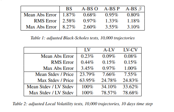
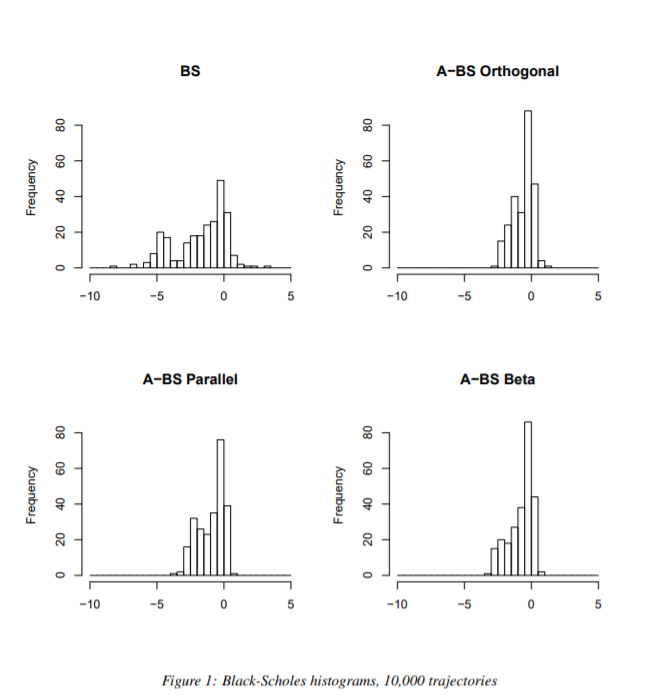
In the table 1, we compare the Black-Scholes price, the adjusted Black-Scholes Orthogonal (A-BS O), the adjusted Black-Scholes Parallel (A-BS O)
and the adjusted Black-Scholes $\beta$ (A-BS $\beta$), each with 10,000 trajectories, to the local volatility reference price. The results on the table are the average of the relative absolute error
(Mean Abs Error), the Root Mean Squared relative error (RMS Error), and the maximal error (Max Abs Error). First, we notice that whatever the strategy, the adjusted prices are closer
to the reference prices than the unadjusted prices, for three different distances, and with a significant improvement. We also notice that the Orthogonal strategy is the best on this portfolio,
and makes the assumption that it should often be the better on secondary market price (thus it should be the default choice). However, it is not necessarily true for the primary price. Indeed, if we
consider for instance a capital protected on the worst performance of two underlyings $S_1, S_2$, whose payoff at $T$ is
In the current market situation, the forwards are likely to be lower than the spots, thus the two adjusters are constant payoffs, equal to $1$. In this case, it is better to use the parallel strategy. Assuming that $\frac{F_1(0, T)}{S_1(0)} \leq \frac{F_2(0, T)}{S_1(0)}$ the corresponding adjusters will be:
$$ \begin{align*} A_1 &= 1 + \max\left(0, \frac{S_1(T)}{S_1(0)} - 1\right)\\ A_2 &= 1 + \max\left(0,\frac{S_1(T)F_2(0, T)}{F_1(0, T)S_2(0)} - 1\right) \end{align*} $$This is obviously a better choice than constant payoffs.
The figure 1 shows the complete relative error distribution (the abscissa is a percentage), and confirms that the adjusted prices are better.
The other results test the efficiency of our adjuster to improve the numerical convergence, and the relevance of using our interpolated market price on the piecewise linearized payoff, versus the use of the initial adjuster payoff, priced within the initial model using finite difference method. Because on the tested portfolio the Orthogonal strategy is the best, we only compare adjusted Local Volatility Orthogonal, standard Local Volatility and Local Volatility with Orthogonal control variables, with 10,000 trajectories and 10 days time step (same discretization scheme) to the reference price.
The table 1 shows the same distance to the expected price as for the Black-Scholes tests. These distances confirm the choice of the adjuster as control variables, because the prices are much closer for the adjusted Local Volatility (A-LV) and the Local Volatility with control variables (LV-CV) than the unadjusted Local Volatility. Furthermore, the distances are almost the same for A-LV and LV-CV, which confirms that we can use our volatility interpolation (including the quanto price approximation) and the piecewise linearization of the payoff to achieve similar results than in a classical control variables algorithm, but the market prices are faster to evaluate than model prices (we recall that for Local Volatility model we must still compute them numerically). The second part of this table shows the averaged standard deviation over price ratio (Mean Stdev / Price) and the maximum value for this ratio (Max Stdev / Price). We recall that this ratio is important as it provides the order of magnitude of the Monte Carlo error. The third part shows the averaged new standard deviation over unadjusted standard deviation ratio (Mean Stdev / LV Stdev) and the maximum value for this ratio, that corresponds to the worst possible improvement of the adjuster. These two standard deviation parts confirms the use of adjusted Local Volatility as a Local Volatility with control variables.
As for Black-Scholes, the figure 2 shows the complete relative error distribution (the abscissa is a percentage), and confirms our results.
8. Conclusion
In this paper, after presenting briefly the standard adjuster approach, we propose a modification of this method implying another choice of the weights of the calibration instruments. We propose to minimize a variance instead of the vega, so that the algorithm corresponds to the control variable method for this choice. We show on a real portfolio that this approach dramatically reduces computational cost, and therefore takes a negligible time of the total pricing time.
Moreover, we present a generic choice of the hedging instruments to use (with three variants to handle multi-underlyings), well suited to equity / FX structured products, making this method fully generic.
Our tests show the efficiency of our enhanced method on a realistic structured product portfolio, priced on the secondary market. They also show that our hedging instruments are a good choice of control variables to reduce the Monte Carlo variance, as we observe an average division by 3 of the observed standard deviation.
References
[AH11] Jesper Andreasen and Brian Norsk Huge. Volatility interpolation. Risk Magazine, pages 76–79, March 2011.
[CM98] Peter Carr and Dilip Madan. Towards a theory of volatility trading. In R.A. Jarrow, editor, Volatility: New Estimation Techniques for Pricing Derivatives, pages 417–427. Risk Publication, 1998.
[Gla04] Paul Glasserman. Control variates. In Monte Carlo Methods in Financial Engineering, pages 185–205. Springer, 2004.
[Hag02] Patrick S. Hagan. Adjusters: Turning good prices into great prices. Wilmott Magazine, pages 56–59, December 2002.
[Kar05] Piotr Karasinski. Mindless fitting. Isaac Newton Institute for Mathemati-cal Sciences, City Event "Modelling Philosophy", 2005.
[KP99] Peter E. Kloeden and Eckhard Platen. Explicit order 2.0 weak schemes. In Numerical Solution of Stochastic Differential Equations, pages 485–488. Springer, corrected third printing edition, 1999.