A possible solution to the spurious oscillations in finite difference methods for Partial Differential Equations

Partial Differential Equation (PDE) solving is an important part of numerical analysis in mathematical finance. The classical approach to solve PDE that appears in finance is to use finite difference method. As most of numerical analysis problems, the goal is to find a solution with an error that converges quickly.

The academic way to achieve this goal is to use Crank-Nicolson to solve our PDE, which provides an “order 2” discretisation scheme in time. However, it appears that in practice, Crank-Nicolson is not that good, especially in the absence of regular initial conditions, and produces some spurious oscillations. The goal of this article is to provide a scheme that is also at “order 2” in time, but which does not produce oscillations.

To that, I will work on a simple case that is easily generalisable. In a first part, I will provide some reminders about finite difference methods for PDE and convergence order. Then, I will explain why Crank-Nicolson can produce such oscillations. Our oscillation free scheme will be presented in the last part.

Before we start, I would like to precise that this article is not about spatial discretisation and boundary conditions.

Reminders about finite difference

The framework

Let $\mathbb E \subset \mathbb R$, $\mathcal F (n) = \{f, f: \mathbb R ^ + \times \mathbb E^n \rightarrow \mathbb R^n\}$.

In this article, I will work on PDE of the following form: [ (*)\left { \begin{array}{lrl} \forall (t, x) \in \mathbb R ^ + \times \mathbb E,& \partial_t u (t, x) & \hspace{-5pt} = a(t, x) \partial^2_x u(t, x) + b(t, x) \partial_x u(t, x) + c(t, x) u(t, x)\
\forall x \in \mathbb E & u(0, x) & \hspace{-5pt} = f(x) \end{array} \right. ] where $a$, $b$ and $c \in \mathcal F(1)$, $a \geq 0$ and $f: \mathbb E \rightarrow \mathbb R$.

We introduce the following convention: let $f\in \mathcal F(1)$, we define \begin{align*} f_n: \mathbb R ^ + \times \mathbb E ^ n & \rightarrow \mathbb R^n\\ t, x & \mapsto (f(t, x_0), ..., f(t, x_{n - 1})) ^ T \end{align*}

and also extend the partial differentiation operators to $f_n \in \mathcal F (n)$:

\begin{align*} \partial_t f_n (t, x) & = (\partial_t f (t, x_0), …, \partial_t f (t, x_{n - 1}))^T\
\partial_x f_n (t, x) & = (\partial_x f (t, x_0), …, \partial_x f (t, x_{n - 1}))^T\
\end{align*}

$(*)$ is then equivalent to: \[ \left \{ \begin{array}{lrl} \forall (t, x) \in \mathbb R ^ + \times \mathbb E^n,& \partial_t u_n (t, x) & \hspace{-5pt} = a_n(t, x)^T I_n \partial^2_x u_n(t, x) + b_n(t, x)^T I_n \partial_x u_n(t, x)\\ && + c_n(t, x)^T I_n u_n(t, x)\\ \forall x \in \mathbb E, & u(0, x) & \hspace{-5pt} = f(x) \end{array} \right. \]

The first line can be rewritten $\partial_t u_n = \mathcal L_n u_n$. To simplify notations, we will mix up both notations when there is no ambiguities.

The method

Our goal is to compute $u(T, x)$ for a particular $T \in \mathbb R^+$. To that, we will in a first step time discretise the problem. Let $(n_x, n_t) \in \mathbb N^2$, $(x_{min}, x_{max}) \in \mathbb E^2$, $\delta x = (x_{max} - x_{min})/(n_x - 1)$ and $\delta t = T/(n_t - 1)$. We define $x \in \mathbb E^n$, $t \in \mathbb R^+$ by $\forall i \in [0; n_x - 1], x_i = x_{min} + i \delta x$ and $\forall i \in [0; n_t - 1], t_i = i \delta t$

Spatial discretisation

The first step consists in discretising the operator $\mathcal L_{n_x}$. To that, we approximate the spatial partial derivatives with finite differences:

\begin{align*} \forall i \in [1; n_x - 2], &\
\partial_x u (t, x_i) & = \frac{u (t, x_{i + 1}) - u(t, x_{i - 1})}{2\delta x} + O (\delta x^2)\
\partial^2_x u (t, x_i) & = \frac{u (t, x_{i + 1}) - 2u(t, x_i) + u(t, x_{i - 1})}{\delta x^2} + O (\delta x^2)\
\end{align*}

thus \begin{align*} \forall i \in [1; n_x - 2], &\
\partial_t u(t, x_i) & = a(t, x_i) \frac{u (t, x_{i + 1}) - 2u(t, x_i) + u(t, x_{i - 1})}{\delta x^2} + b(t, x_i) \frac{u (t, x_{i + 1}) - u(t, x_{i - 1})}{2\delta x}\
& + c(t, x_i) u(t, x_i) + O (\delta x^2)\

& = \left(\frac{a(t, x_i)}{\delta x ^ 2} - \frac{b(t, x_i)}{2\delta x}\right)u(t, x_{i - 1}) + \left(c(t, x_i) - 2 \frac{a(t, x_i)}{\delta x ^ 2} \right)u(t, x_i)\\
  & + \left(\frac{a(t, x_i)}{\delta x ^ 2} + \frac{b(t, x_i)}{2\delta x}\right)u(t, x_{i + 1}) + O (\delta x^2)

\end{align*}

Now, we have to discretise in the boundary. To that, we assume that $\partial^2_xu(t, x_0) = \partial^2_xu(t, x_{n_x - 1}) = 0$ (I take simple boundary conditions, as this is not the purpose of this article). We can write: \[ \partial_x u(t, x_0) = \frac{u(t, x_1) - u(t, x_0)}{\delta x} + O(\delta x), \hspace{10pt} \partial_x u(t, x_{n_x - 1}) = \frac{u(t, x_{n_x - 1}) - u(t, x_{n_x - 2})}{\delta x} + O(\delta x) \]

what leads to

\begin{align*} \partial_t u (t, x_0) & = \left(c(t, x_0) - \frac{b(t, x_0)}{\delta x}\right) u(t, x_0) + \frac{b(t, x_0)}{\delta x} u(t, x_1) + O(\delta x)\
\partial_t u (t, x_{n_x - 1}) & = - \frac{b(t, x_{n_x - 1})}{\delta x}u(t, x_{n_x - 2}) + \left( \frac{b(t, x_{n_x - 1})}{\delta x} + c(t, x_{n_x - 1}) \right) u(t, x_{n_x - 1}) + O(\delta x) \end{align*}

Let $\Delta x^2 \in \mathbb R ^ {n_x}$ defined by $\forall i \in [1; n_x - 2], (\Delta x^2)_i = \delta_x ^ 2, (\Delta x^2)_0 = (\Delta x^2)_{n_x - 1} = \delta x$.

We can write: [ \partial_t u_{n_x} (t, x) = \mathrm L_{n_x} (t, x) u_{n_x}(t, x) + O(\Delta x^2) \hspace{50pt} (1) ]

where $\mathrm L_{n_x}(t, x)$ in a $n_x \times n_x$ tridiagonal real matrix defined by

\begin{align*} \mathrm L_{n_x}(t, x)_{0, 0} & = c(t, x_0) - \frac{b(t, x_0)}{\delta x}\
\mathrm L_{n_x}(t, x)_{0, 1} & = \frac{b(t, x_0)}{\delta x} \end{align*}

\begin{align*} \mathrm L_{n_x}(t, x)_{i, i - 1} & = \frac{a(t, x_i)}{\delta x ^ 2} - \frac{b(t, x_i)}{2\delta x}\
\mathrm L_{n_x}(t, x)_{i, i} &= c(t, x_i) - 2 \frac{a(t, x_i)}{\delta x ^ 2}\
\mathrm L_{n_x}(t, x)_{i, i + 1} &= \frac{a(t, x_i)}{\delta x ^ 2} + \frac{b(t, x_i)}{2\delta x} \end{align*}

\begin{align*} \mathrm L_{n_x}(t, x)_{n_x - 1, n_x - 2} & = - \frac{b(t, x_{n_x - 1})}{\delta x}\
\mathrm L_{n_x}(t, x)_{n_x - 1, n_x - 1} &= \frac{b(t, x_{n_x - 1})}{\delta x} + c(t, x_{n_x - 1}) \end{align*} </br/>

time discretisation

Now that we rewrote our problem as $(1)$, we are in a classical differential equation of the form $\partial_t f(t) = g(t)$. Classical ways to solve this kind of equation are the Euler schemes (implicit and explicit). The implicit scheme uses $f(t + \delta t) = f(t) + g(t) \delta t + O (\delta t ^2)$, and the explicit $f(t + \delta t) = f(t) - g (t + \delta t) \delta t + O (\delta t^2)$.
Let's return to $(1)$:

Let $\tilde u$ defined by the following induction (Explicit Euler scheme (EE)):

\begin{align*} \tilde u_0 & = u(0, x)\
\tilde u_{i + 1} & = \tilde u_i + \mathrm L(t_i, x) \tilde u_i \delta t = (I + \delta t \mathrm L (t_i, x)) \tilde u_i \end{align*}

We can show that $\tilde u_{n_t - 1} - u(T, x) = O(\Delta x ^ 2 + \delta t \mathbf 1)$:

To that, we show by an induction $P(i): \tilde u_i - u(t_i, x) = O(i\delta t \Delta x ^ 2 + i \delta t ^ 2 \mathbf 1)$:
the case $i = 0$ is trivial as the equality hold by construction (without big $O$).

We suppose $P(i)$:

\begin{align*} \partial_t u(t_i, x) & = \mathrm L(t_i, x)u(t_i, x) + O(\Delta x^2)\
\Rightarrow u(t_{i + 1}, x) & = (I + \delta t \mathrm L(t_i, x)) u (t_i, x) + O(\delta t \Delta x^2 + \delta t\mathbf 1)\
& = (I + \delta t \mathrm L(t_i, x)) (\tilde u_i + O(i \delta t \Delta x ^ 2 + i \delta t ^ 2 \mathbf 1)) + O(\delta t \Delta x^2 + \delta t\mathbf 1)\
& = (I + \delta t \mathrm L(t_i, x)) \tilde u_i + O((i+1) \delta t \Delta x ^ 2 + (i+1) \delta t ^ 2 \mathbf 1)\
\Rightarrow \tilde u_{i + 1} - u(t_{i + 1}, x) & = O\left((i+1) \delta t \Delta x ^ 2 + (i+1) \delta t ^ 2 \mathbf 1\right) \end{align*}

We showed $P(0)$ and $P(i) \Rightarrow P(i+1)$, then $\forall i \in \mathbb N, P(i)$. In particular, $P(n_t - 1)$:

[ \tilde u_{n_t - 1} = u(t_{n_t - 1}, x) + O((n_t - 1)\delta t \Delta x ^ 2 + (n_t - 1) \delta t ^ 2 \mathbf 1) ]

Using $n_t - 1 = \frac{T}{\delta T}$, we have

[ u(T, x) - \tilde u_{n_t - 1} = O(\Delta x ^ 2 + \delta t \mathbf 1) ]

We note that the error at $T$ is of order 2, while it is of order 3 between $t$ and $t + \delta t$. In general, when the error is of order $n + 1$ on a time step, it will be at order $n$ at $T$.

If we defined $\tilde u$ by the following induction (Implicit Euler scheme (IE)), we have the same results using a similar demonstration:

\begin{align*} \tilde u_0 & = u(0, x)\
\tilde u_{i + 1} & = \tilde u_i - \mathrm L(t_{i + 1}, x) \tilde u_{i + 1} \delta t\
\Rightarrow \tilde u_{i + 1} & = (I - \delta t \mathrm L (t_{i+1}, x))^{-1} \tilde u_i \end{align*}

Now, we can use a mixture of the two scheme to try to increase the time order: \begin{align*} \tilde u_0 & = u(0, x)\
\tilde u_{i + 1} & = \tilde u_i - \theta \mathrm L(t_{i + 1}, x) \tilde u_{i + 1} \delta t + (1 - \theta) \mathrm L(t_i, x)\tilde u_i \
\Rightarrow \tilde u_{i + 1} & = (I - \theta \delta t \mathrm L (t_{i+1}, x))^{-1} (I + (1 - \theta)\delta t \mathrm L (t_i, x))\tilde u_i \end{align*}

It is easy to show that taking $\theta = \frac{1}{2}$, we have an order 2 time scheme:

\begin{align*} u(t + \delta t, x) & = u(t, x) + \delta t \partial_t u(t, x) + \frac{\delta t^2}{2} \partial_t ^ 2 u(t, x) + O(\delta t ^ 3)\
u(t, x) & = u(t + \delta t, x) - \delta t \partial_t u(t + \delta t, x) + \frac{\delta t^2}{2} \partial_t ^ 2 u(t + \delta t, x) + O(\delta t ^ 3) \end{align*}

We rewrite the second line: \begin{align*} u(t + \delta t, x) & = u(t, x) + \delta t \partial_t u(t + \delta t, x) - \frac{\delta t^2}{2} \partial_t ^ 2 u(t + \delta t, x) + O(\delta t ^ 3)\
& = u(t, x) + \delta t \partial_t u(t + \delta t, x) - \frac{\delta t^2}{2} (\partial_t ^ 2 u(t, x) + O (\delta t)) + O(\delta t ^ 3)\
& = u(t, x) + \delta t \partial_t u(t + \delta t, x) - \frac{\delta t^2}{2} \partial_t ^ 2 u(t, x) + O(\delta t ^ 3)\
\end{align*}

applied on a $\theta$ scheme:

[ u(t, x) + \theta \delta t \partial_t u (t + \delta t, x) + (1 - \theta) \delta t \partial_t u(t, x) - u(t + \delta t, x) = (2\theta - 1)\frac{\delta t^2}{2}\partial_t^2u(t, x) + O(\delta t ^ 3) ]

taking $\theta = \frac{1}{2}$:

[ u(t, x) + \frac{1}{2} \delta t \partial_t u (t + \delta t, x) + \frac{1}{2}\delta t \partial_t u(t, x) - u(t + \delta t, x) = O(\delta t ^ 3) ]

what leads to an order 2 in time scheme. This scheme is the so called Crank-Nicolson scheme. </br/></br/></br/>

We can also remark that a time step $\delta t$ of a $\theta$-scheme is a EE time step $(1 - \theta)\delta t$ followed by a IE time step $\theta \delta t$. In the particular Crank-Nicolson case, this is a EE half time step followed by a IE half time step.

What's wrong with Crank-Nicolson ?

The undesired behavior of Crank-Nicolson scheme comes from the Explicit Euler part, and each $\theta$ scheme, will have the same behavior (except the case $\theta = 1$), as each step of a $\theta$ scheme can be decomposed into an explicit step followed by an implicit. To see the problem, we consider the simple following PDE:

\begin{align*} \forall (t, x) \in \mathbb R^+ \times \mathbb R, \partial_t u(t, x) & = a \partial_x ^ 2 u(t, x) + b \partial_x u(t, x) + c u(t, x)\
\forall x \in \mathbb R, u(0, x) = \mathbf 1_{x > 0} \end{align*}

Where $a, b, c \in \mathbb R^+ \times \mathbb R \times \mathbb R$. We discretise $x$ and $t$ as in the previous section. Let $i_0 \in [0; n_x - 1]$ such that $x_{i_0} \leq 0 \lt x_{i_0+1}$. We note that $\forall i \leq i_0, \tilde u^0_i = 0$ and $\forall i \gt i_0, \tilde u^0_i = 1$. Let’s look at the value of u near $0$ after the first step:

\begin{align*} \tilde u ^ 1_{i_0} & = \tilde u ^ 0_{i_0} + \delta t \left(a \frac{\tilde u^0_{i_0 + 1} + \tilde u^0_{i_0 - 1} - 2 \tilde u^0_{i_0}}{\delta x ^ 2} + b\frac{\tilde u^0_{i_0 + 1} - \tilde u^0_{i_0 - 1}}{2\delta x} + c \tilde u^0_{i_0}\right)\
& = \delta t \left(a \frac{1}{\delta x ^ 2} + b\frac{1}{2\delta x}\right) \end{align*}

and

\begin{align*} \tilde u ^ 1_{i_0 + 1} & = \tilde u ^ 0_{i_0 + 1} + \delta t \left(a \frac{\tilde u^0_{i_0 + 2} + \tilde u^0_{i_0} - 2 \tilde u^0_{i_0 + 1}}{\delta x ^ 2} + b\frac{\tilde u^0_{i_0 + 2} - \tilde u^0_{i_0}}{2\delta x} + c \tilde u^0_{i_0 + 1}\right)\
& = 1 + \delta t \left(a \frac{-1}{\delta x ^ 2} + b\frac{1}{2\delta x} + c\right) \end{align*}

We can reasonably think that for a small $\delta t$, $u(\delta t, x_{i_0}) \leq u(\delta t, x_{i_0 + 1})$

\begin{align*} \tilde u ^ 1_{i_0 + 1} - \tilde u ^ 1_{i_0} &= 1 + \delta t \left(a \frac{-1}{\delta x ^ 2} + b\frac{1}{2\delta x} + c\right) - \delta t \left(a \frac{1}{\delta x ^ 2} + b\frac{1}{2\delta x}\right)\
& = 1 - \delta t \left( \frac{2a}{\delta x^2} - c \right)\
\tilde u ^ 1_{i_0 + 1} - \tilde u ^ 1_{i_0} \geq 0 & \Leftrightarrow 1 \geq \delta t \left( \frac{2a}{\delta x^2} - c \right) \end{align*}

The previous condition can be easily violated if $\delta x ^ 2 \ll \delta t$. It implies that if we decrease $\delta x$ with fixed $\delta t$, spurious oscillations will appear, while a good scheme should increase precision when $\delta t$ or $\delta x$ decrease.

We remind one more time that the Crank-Nicolson scheme is nothing but a EE half time step followed by a IE half time step. The condition for the Crank-Nicolson to bad behave is then the same, replacing $\delta t$ with $\frac{\delta t}{2}$, ie if $1 < \delta t \left( \frac{a}{\delta x^2} - \frac{c}{2} \right)$, the Crank-Nicolson scheme will oscillate.

Another time order 2 scheme that does not use explicit time step

Our goal is to find a scheme with a time order 2, without using explicit scheme. The idea is to use extrapolation method, in particular the Richardson Extrapolation. What we will do is to take a convex combination of the solution obtained with a time step $\delta t$ and the one with two time step $\frac{\delta t}{2}$, and cancel the smallest order term of the error.

We define our scheme with the following induction:

\begin{align*} \tilde u_0 & = u(0, x)\
v_{i + 1} & = \left(I - \delta t \mathrm L (t_{i+1}, x)\right)^{-1} \tilde u_i\
w_{i + 1} & = \left(I - \frac{\delta t}{2} \mathrm L (t_{i+1}, x)\right)^{-1} \left(I - \frac{\delta t}{2} \mathrm L (t_i + \frac{\delta t}{2}, x)\right)^{-1} \tilde u_i\
\tilde u_{i + 1} & = (1 - \omega) v_{i + 1} + \omega w_{i + 1}\
\end{align*}

Let's examine the error on the two implicit scheme, to find the $\omega$ that will cancel the smallest order term of the error:

Error on the IE time step:

\begin{align*} & u(t + \delta t, x) = u(t, x) + \delta t \partial_t u(t + \delta t, x) - \frac{\delta t^2}{2} \partial_t^2u(t + \delta t, x) + O (\delta t^3)\
& \Rightarrow u(t, x) + \delta t \partial_t u(t + \delta t, x) - u(t + \delta t, x) = \frac{\delta t^2}{2} \partial_t^2u(t + \delta t, x) + O (\delta t^3) \end{align*}

Error made on the two half IE time steps:

[ \left{\begin{array}{rl} u(t + \frac{\delta t}{2}, x) & \hspace{-5pt} = u(t, x) + \frac{\delta t}{2} \partial_t u(t + \frac{\delta t}{2}, x) - \frac{\delta t^2}{8} \partial_t^2u(t + \frac{\delta t}{2}) + O (\delta t^3)\
u(t + \delta t, x) & \hspace{-5pt} = u(t + \frac{\delta t}{2}, x) + \frac{\delta t}{2} \partial_t u(t + \delta t, x) - \frac{\delta t^2}{8} \partial_t^2u(t + \delta t, x) + O (\delta t^3)\
\end{array}\right.\
\] \begin{align*} \Rightarrow e_{1/2} &= u(t, x) + \frac{\delta t}{2} \partial_t u(t + \frac{\delta t}{2}, x) + \frac{\delta t}{2} \partial_t u (t + \delta t, x) - u(t + \delta t, x)\
&= \frac{\delta t ^ 2}{8} (\partial_t^2u(t + \delta t, x) + \partial_t^2u(t + \frac{\delta t}{2}, x)) + O(\delta t^3)\
&= \frac{\delta t ^ 2}{8} (\partial_t^2u(t + \delta t, x) + (\partial_t^2u(t + \delta t, x) + O(\delta t))) + O(\delta t^3)\
&= \frac{\delta t ^ 2}{4} \partial_t^2u(t + \delta t, x) + O(\delta t^3) \end{align*}

The error on our new scheme is then:

\begin{align*} e_\omega & = (1 - \omega)(u(t, x) + \delta t \partial_t u(t + \delta t, x)) + \omega \left(u(t, x) + \frac{\delta t}{2} \partial_t u(t + \frac{\delta t}{2}, x) + \frac{\delta t}{2} \partial_t u (t + \delta t, x)\right)\
& \hspace{10pt} - u(t + \delta t, x) \
& = (1-\omega) \frac{\delta t^2}{2}\partial_t^2u(t + \delta t, x) + \omega \frac{\delta t^2}{4}\partial_t^2u(t + \delta t, x) + O(\delta t ^ 3)\
& = \frac{\delta t^2}{4}\partial_t^2u(t + \delta t, x)(2 - \omega) + O(\delta t ^ 3) \end{align*}

The value of $\omega$ that cancel the order 2 term is $2$. Then, taking $\omega = 2$ leads to a time order 2 time scheme. This scheme is:

Here we are ! We found a scheme that is order 2 in time without using explicit time step. Let's experiment all that in the next section.

Numerical examples

For the numerical examples, I will work with the basic heat equation

[ \partial_t u(t, x) = \partial_x ^ 2 u(t, x) ]

with the initial condition $u(0, x) = \mathbf 1_{x > 0}$. Surprising, isn’t it ?

I will start expressing analytically the solution at $T \in \mathbb R^+$. Using the Feynman-Kac formula on $v$ defined by $v(t, x) = u(T - t, x)$, we have:

\begin{align*} \forall x \in \mathbb R, u(T, x) & = \mathbb E [\mathbf 1_{X(T) > 0} | X(0) = x]\
dX(t) &= \sqrt 2 dW(t) \mbox{ where $W$ is a standard brownian motion}\
\end{align*}

Then:

\begin{align*} \forall x \in \mathbb R, u(T, x) &= \mathbb E [\mathbf 1_{x + \sqrt 2 W(T) \gt 0}]\
& = \mathbb P (x + \sqrt 2 W(T) \gt 0)\
& = \mathbb P (\sqrt {2T} Z \gt -x) \mbox{ where $Z \sim \mathcal N(0, 1)$}\
& = \mathbb P (\sqrt {2T} Z \lt x) \end{align*}

We can conclude that $u(T, x) = \phi \left(\frac{x}{\sqrt {2T}}\right)$ where $\phi$ is the cumulative distribution function of the standard normal distribution.

Before showing some graphics, I will briefly discuss the choice of $x_{min}$ and $x_{max}$. First, we can remark that the problem is almost symmetric. Thus, taking $x_{min} = -x_{max}$ is a good idea. To preserve the symmetry, we can also take $n_x$ even, then $0$ will fall between two grid points, and the initial vector $\tilde u_0$ will be symmetric.

The last thing we can remark is on the probabilistic formulation of the PDE: the value depends on a Gaussian law, that is highly concentrated into a small interval. For example, if we call $\sigma$ the standard deviation of the concerned Gaussian law, the random variates will leave the interval $[-5\sigma; 5\sigma]$ with a probability lower than $10^{-6}$.

Thus, I take $x_{max} = 5\sqrt{2T}$ for my example, what will cause the boundary error to be negligible, according to my previous remark.

I briefly provide all the fixed parameters I used for my test:

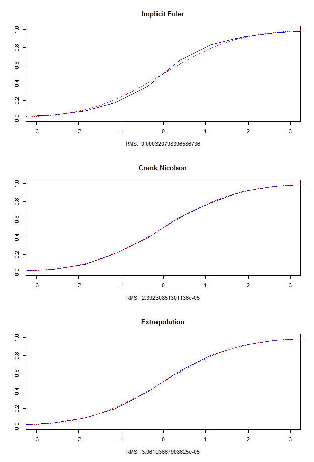
\begin{align*} T & = 1\
x_{min} &= -5\sqrt 2\
x_{max} &= 5\sqrt 2 \end{align*}

For each test case, I draw three graphics: one for Implicit Euler, one for Crank-Nicolson and one for the scheme obtained with Richardson Extrapolation. On each graphic, the dotted red line is the exact value, and the blue line is the value obtained with the corresponding scheme. There is also on the bottom of each graphic a Root Mean Squared error that measure the error done by the scheme. The formula to compute the RMS is $\frac{1}{n_x - 1}\sum_{i=0}^{n_x - 1} (\tilde u ^ {n_t}_i - u(T, x_i))^2$.

Test case I: $n_t = 3, n_x = 20 \hspace{5pt} \left(\delta t = \frac{1}{2}, \delta x \approx 0.74\right)$:

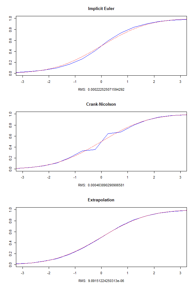
Test case II: $n_t = 3, n_x = 30 \hspace{5pt} \left(\delta t = \frac{1}{2}, \delta x \approx 0.49\right)$:

Test case III: $n_t = 2, n_x = 200 \hspace{5pt} \left(\delta t = 1, \delta x \approx 0.07\right)$:

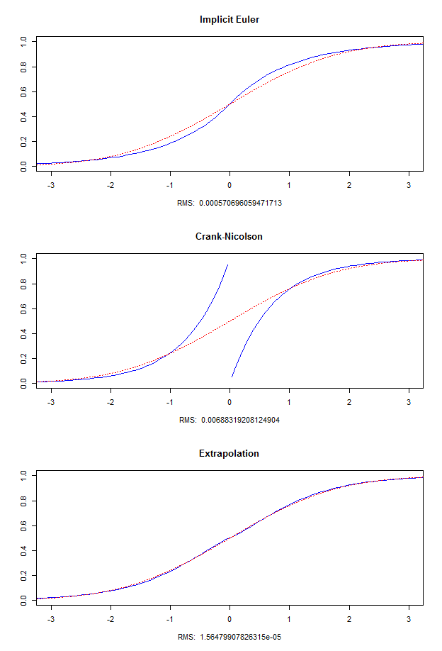
On the test case I, we see that the error is of the same order in the case of Crank-Nicolson and Extrapolation, and is bigger in the Implicit Euler case. On the test case II (lower space step), we see Crank-Nicolson has a bad behavior, while Implicit Euler and Extrapolation are better than in the test case II, and Extrapolation is still the best. The test case III is an extreme test case to show how wrong can be Crank-Nicolson, and how fast the scheme using extrapolation converge in time.

Conclusion

After a brief study of classical PDE finite difference scheme, I showed that the Crank-Nicolson one, supposed to be a good one, behaves badly in some cases, due to the explicit part of the scheme. I proposed a new scheme based on Richardson Extrapolation that has the same theoretical order in space that the Crank-Nicolson one, but that doesn't oscillate. The theoretical aspect is confirmed by the numerical results I presented in the last part. We can also note that the method can be extended to multi space dimension PDE with little effort.

I invite the reader who wants to go further on this topic to read:

A possible solution to the spurious oscillations in finite difference methods for Partial Differential Equations.

Vivien Begot