Poisson distribution is a classical distribution that often appears in mathematical finance, like in jump diffusion. In this article, I will present an efficient simulation method under the constraint to use only one random variate per simulation.
This constraint is useful when using low-discrepancy sequence for instance.
The Poisson distribution
The Poisson distribution with parameter is a discrete probability distribution, with positive values and whose probability mass function is given by
Its mean is and its variance is . For the following, we provide also its skewness and its excess kurtosis :
We note that Poisson variable (with parameters ) can also be seen as the value at of a counting process whose jumps are of size 1 and whose jump time are separated by an exponential distribution (with parameters ).
Let be such a process, with its jump times. where . Then, and . We have
This remark provides a first idea to create a naive Poisson distribution simulation method (the exponential distribution is easy to simulate).
Naive Poisson distribution simulation methods
Using the previous remark, we can easily provide an algorithm to simulate the Poisson distribution:
tau = 0
N = -1
while (tau <= 1)
{
    E = simulate_exp(lambda)
    tau = Tau + E
    N = N + 1
}
N
But this algorithm violates our constraint. Indeed, most of the time we will simulate more than one random variable. Additionally, we don’t even know in advance how many variables we need.
Let’s return to our constraint. The easier way to respect it is to use inversion algorithm. In this case, we have to simulate only one uniform variable per Poisson variable. Let be the cumulative distribution function of a discrete variable (and its probability mass function), the quantile function of defined by
and let be a uniform variable. Then, is distributed.
Proof:
We can then apply this result to our case, and have a good idea to start. Now, the difficulty is to find an efficient way to compute the cumulative distribution function of a Poisson distribution. As we are still in the “naive simulation methods” part, we will see the most basic way to achieve this goal that will be used to benchmark the efficient solution we will propose later. To do that, we simply compute the quantile function using a basic search from until , or just until (as we perform an increasing search, and is an increasing function). We use to efficiently compute and . We propose then the following algorithm to compute (Naive Simulation):
Q = function(lambda, u)
{
    f = exp (-lambda)
    F = f
    k = 1
    while (F < u)
    {
        f = lambda / k * f
        F = F + f
        k = k + 1
    }
    k - 1
}
The expected complexity of this algorithm is (the number of iterations is a Poisson random variable). Then, the bigger is, the less efficient this algorithm is.
The method
The proposed method is still based on a research of such that , but now instead of starting at , we start at , where is an easily computable approximation of the quantile function of a Poisson law with parameter . Such an approximation can be found using the Cornish-Fisher expansion.
The Cornish-Fisher expansion
The Cornish-Fisher expansion is a formula that approximates quantile (or realization) of any variable using standard Gaussian variable, based on the cumulant. In our case, we use the approximation with the 4 first cumulants, what leads to:
where is a variable we want to approximate with mean and variance, a standard Gaussian variable, the skewness of and the excess kurtosis of . This formula can be adapted with with mean and variance, applying the formula to , and using the fact that skewness and excess kurtosis are invariant by affine transformation:
if we note the quantile function of and the quantile function of a standard Gaussian variable, we have:
We note that the right term of this formula must be a strictly increasing function for the approximation to hold.
Application to the Poisson distribution
We can use the previous formula in the case of the Poisson distribution:
In our case, the function we want to approximate has positive integer value. Then, we set
where is the positive part of the rounding of , ie .
Here are some examples of the precision of our approximation (the black curve is the exact function and the red one the approximated function):
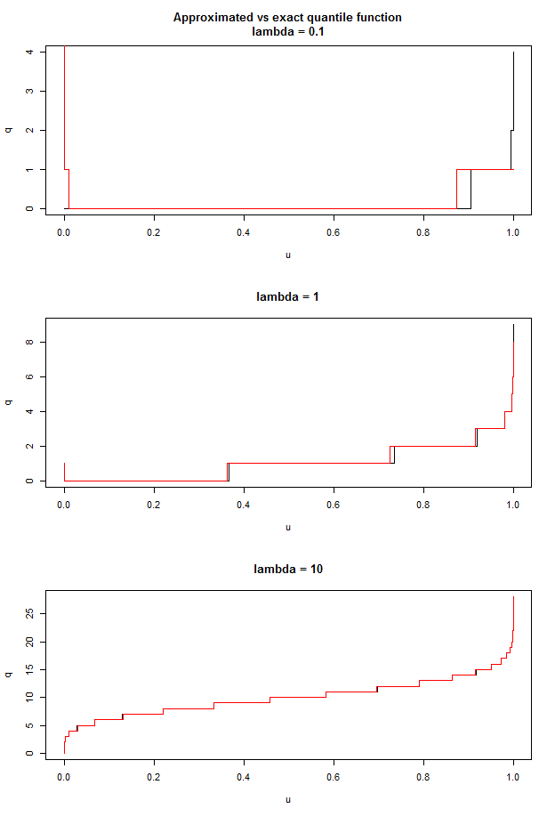
We see that:
- the bigger is, the more the approximation is precise
- the approximation is poor near
- except the case close to , the error is rarely bigger than one
The second point can be easily fixed using the approximation for , and for . Let’s have a look at the corresponding new approximation:
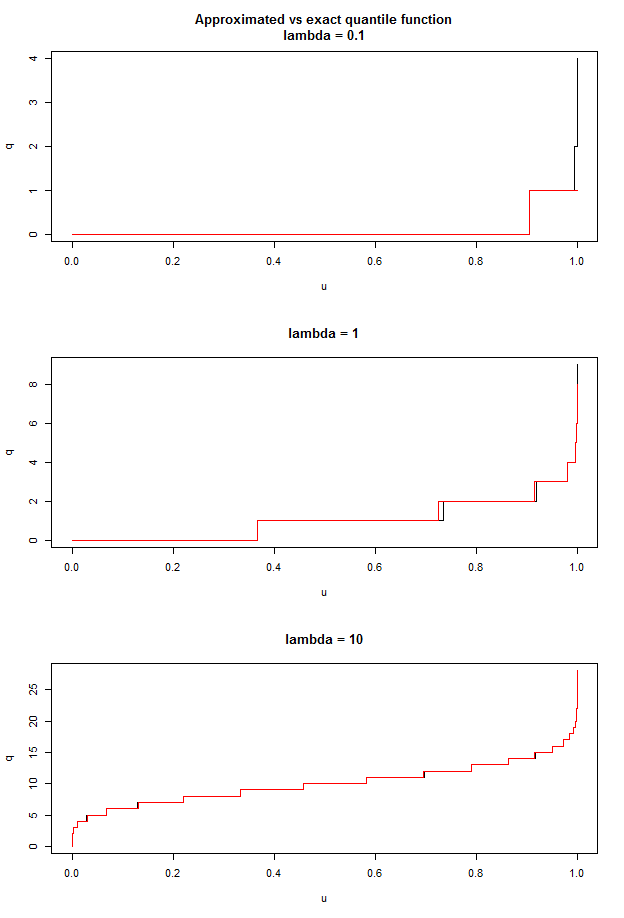
This approximation is satisfying for a first guess in a search algorithm.
The complete method
The goal is to find such that . As told previously, we perform a search from , or more precisely we perform the search for (and return otherwise).
The last issue we have to solve at this point is the computation of , that has a linear complexity in its first argument if computed each time. The solution is to precompute in an array the for . We note that this solution is only relevant when we have many computations of for a fixed , ie when we have to simulate a lot of Poisson variables with the same intensity. This is the case in Monte Carlo method for instance. There are many ways to choose to control the error. For instance, we can fix , and choose such that , or . A last trick we can use to improve a little the algorithm is to hard-code the first cases using the precomputed array (the first must be in all case hard-coded due to the poor efficiency of the approximation near for small ). It will be particularly efficient with small .
The final algorithm is then (Cornish-Fisher Simulation):
buildQ = function(lambda)
{
    F = precompute_F (lambda)
    F0 = F[0]
    F1 = F[1]
    ...
    n = length (F)
    function (u)
    {
        if (u <= F0) 0
        else if (u <= F1) 1
        ...
        else
        {
            q = gaussian_quantile(u)
            bar_q = q * sqrt(lambda) + (q^2 - 1) / 6
                  + (q - q^3) / (72 * sqrt(lambda)) + lambda
            bar_q = max(0, floor(bar_q + 0.5))
            if (bar_q >= n)
                bar_q
            else if (u <= F[bar_q - 1])
                decreasing search from bar_q - 1
            else if (F[bar_q] < u)
                increasing search from bar_q + 1
            else bar_q
        }
    }
}
Remark: The inverse of the Gaussian cumulative distribution function can replaced with an approximation (e.g. using this approximation for ).
Results and conclusion
I implemented the two algorithm in R, then the timing can be high, but what matter is the ratio between methods. In the (CFS) method, I hard-coded the 5 first cases. In all test case, I take numbers uniformly distributed between 0 and . Here are my results:
| λ | 0.01 | 0.1 | 0.5 | 1 | 5 | 10 | 50 | 100 |
| NS | 0.34 | 0.38 | 0.45 | 0.56 | 1.44 | 2.40 | 10.70 | 20.80 |
| CFS | 0.20 | 0.21 | 0.22 | 0.25 | 0.94 | 1.33 | 1.35 | 1.36 |
| Ratio | 1.67 | 1.81 | 2.00 | 2.24 | 1.54 | 1.80 | 7.91 | 15.24 |
We see that for all , the (CFS) method is faster than the (NS) method. For small , it is due to the hard-coding of the first few tests. For big , it is due to the constant complexity of (CFS), while the complexity of (NS) is in average.
The (CFS) method is designed to work very well for simulation of a large number of Poisson variables with the same intensity. However, it will be particularly inefficient when intensities are not constant. An example of problems that can be solved using this method are Monte Carlo method when some underlying distributions are Poisson law. This is the case for instance for pricing in jump models with compound Poisson process, like Merton or Bates models. The implementation in LexiFi of these two models use the (CFS) method, which leads to an efficient Monte Carlo method.