Building the (zero-coupon) yield curve is the first step in most of the financial modeling problems. We will present in this post how the yield curve is computed into LexiFi Apropos, and how we make our algorithm generic so that it can easily be used to compute different kinds of yield curves or solve different problems.
Simple formulation of the problem
We assume a simplified market where we can observe the Deposit Rates and the Swap Rates. We also assume there is only one curve.
Let $P(T)$ be today’s value of the $T$-maturing bond. Building the yield curve means finding a function $P$ that allows
to match the market price of Deposit Rates and Swap Rates.
Let $L(T)$ be the value of the $T$-maturing deposit. We have:
\[ L(T) = \frac{1}{T}\left[\frac{1}{P(T)} - 1\right] \]Let $S(T)$ be the value of the $T$-maturing swap rate. We assume that the fix leg period of the swap is $\delta$. We have:
\[ S(T) = \frac{1 - P(T)}{\delta \sum_{i = 1}^{T/\delta} P(\delta i)} \]We observe on the market $L(t_i)$ for $i \in [0; m - 1]$ and $S(t_i)$ for $i \in [m; n - 1]$, where $t_0 < t_1 < ... < t_{n-1}$
Resolution of the simple problem
We define $I_i$:
\[ I_i=\left\{ \begin{array}{ll} L(t_i) & \forall i \in [0; m - 1]\\ S(t_i) & \forall i \in [m; n - 1]\\ \end{array} \right. \]We note that $I_i$ only depends on $P(t)$ for $t \leq t_i$.
The problem can then be solved by using a “bootstrap” procedure:
- find $P$ on $[0; t_0]$ that allows to match $I_0$
- find $P$ on $[t_0; t_1]$ that allows to match $I_1$, knowing $P$ on $[0; t_0]$
- ...
- find $P$ on $[t_{n - 2}; t_{n - 1}]$ that allows to match $I_{n - 1}$, knowing $P$ on $[0; t_{n - 2}]$
The previous problem has an infinity of solutions. To avoid that, we can use a parametrisation $\mathcal P_i$ such as $P(t) = \mathcal P_i(p_0, p_1, ...p_i, t)$ for $t \leq t_i$.
Let $I_i^{mkt}$ be the observed value of the $i$-th instrument. We define $\mathcal I_i(P)$ the value of the $i$-th instrument if the curve is $P$.
The problem is now:
- find $p_0$ so that $\mathcal I_0 (\mathcal P_0(p_0, \cdot)) = I_0^{mkt}$
- find $p_1$ so that $\mathcal I_1 (\mathcal P_1(p_0, p_1, \cdot)) = I_1^{mkt}$
- ...
- find $p_{n - 1}$ so that $\mathcal I_{n - 1} (\mathcal P_{n - 1}(p_0, p_1, ..., p_{n - 1}, \cdot)) = I_{n - 1}^{mkt}$
- set $\forall t, P(t) = \mathcal P_{n-1}(p_0, p_1, ..., p_{n - 1}, t)$
Now, we need to find a good parametrisation for $\mathcal P$. In order to do that, we recall that there are some natural ways of rewriting the curve defining the yield:
$$ \begin{align*} r(t) &= -\frac{log(P(t))}{t}\\ \Rightarrow P(t) &= e^{-r(t)t} \end{align*} $$or the instantaneous forward rate:
$$ \begin{align*} f(t) &= -\partial_t log(P(t))\\ \Rightarrow P(t) &= e^{-\int_0^tf(s)ds} \end{align*} $$Thus, one needs to parametrise only $r$ or $f$, using for instance a piecewise constant or a piecewise affine term-structure.
Remark on possible parametrisations
The use of a piecewise affine function for $f$ seems a good idea as it leads to a $\mathcal C^1$ function $P$. However, the resulting function can be “unstable”, because the mid value depends on the left value: a small perturbation on the left value will be compensated by a perturbation on the right value, in the opposite direction (and will propagate to the last date). On the other hand, the use of a piecewise constant function for $f$ leads to a only $\mathcal C^0$ function $P$, but with a more stable result as in this case the mid values depend only on the left value (then a small perturbation on the beginning of the curve doesn’t propagate itself).
At first, it seems that there is a trade-off between curve smoothness and curve stability. However, it can be easily solved by using a two step building procedure:
- Step 1: Bootstrap using a piecewise constant instantaneous forward.
- Step 2: Keep the bootstrapped values on the pillar dates (the dates on which $P$ is needed to match the market prices), and interpolate between these dates using a monotonic cubic spline for the yield.
This procedure leads to a stable and smooth curve, but requires one more step.
Proposed parametrisation of the curve
Even though the two step procedure is a good choice, we propose a different method, that is only one step, and achieves the same smoothness and stability. For that, we use a locally affine parametrisation of the instantaneous forward $f$, ie given a level $\epsilon$, $f$ is affine from $t_{i-1}$ to $t_{i - 1} + \epsilon (t_i - t_{i - 1})$ and constant after (until $t_i$):
- $f_{i - 1} := f(t_{i-1})$
- $f_i := f(t_i)$
- $f(t) = f_{i - 1} + (f_i - f_{i - 1})\frac{t - t_{i-1}}{\epsilon (t_i - t_{i-1})}$ for $t \in [t_{i - 1}; t_{i - 1} + \epsilon (t_i - t_{i - 1})]$
- $f(t) = f_i$ for $t \in [t_{i - 1} + \epsilon (t_i - t_{i - 1}); t_i]$
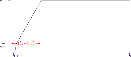
This parametrisation leads to a $\mathcal C^0$ function $f$, and then $\mathcal C^1$ functions $r$ and $P$. The stability is achieved when we choose a small value for $\epsilon$, as $f$ is almost piecewise constant in this case.
Generalisation
In finance, there are a lot of problems that require bootstrapping a function of the form $e^{-\int_0^tf(s)ds}$. Then it can be a good idea to think about a generic implementation of this problem solving. In order to do that, we start by defining simple algebra for formula to bootstrap:
Expression $\rightarrow$ Expression + Expression
Expression $\rightarrow$ Expression * Expression
Expression $\rightarrow$ (Expression)
Expression $\rightarrow$ float
Expression $\rightarrow$ P(date, date)
Such as
\[
P(t_0, t_1) = e^{-\int_{t_0}^{t_1}f(s)ds}
\]
Expression $\rightarrow$ Expression * Expression
Expression $\rightarrow$ (Expression)
Expression $\rightarrow$ float
Expression $\rightarrow$ P(date, date)
such a grammar can be defined using an Algebraic Data Type:
type expression =
    | Add of expression * expression
    | Mul of expression * expression
    | Cst of float
    | P of float * float
As an example, the expression to solve for the deposit is:
Add (Mul (Cst (1 / T), Add(P(T, 0), Cst (-1))),
          Cst (-L(T)))
And for the bootstrap to be possible, we need to write an evaluation function that takes the function $p$ to bootstrap as an input:
let rec eval exn p =
  match exn with
  | Add (e1, e2) -> eval e1 p +. eval e2 p
  | Mul (e1, e2) -> eval e1 p *. eval e2 p
  | Cst x -> x
  | P (t0, t1) -> p t1 /. p t0
To get an efficient implementation, we need two more functions. First, a simplification function that evaluates each occurrence of P(t0, t1) in the expression when t0 and t1 are lower than $T$ (with $T$ set to $t_{i-1}$ when finding P between $t_{i-1}$ and $t_i$)). Then, a factorisation function that tries to write the simplified expression in the form A P(t0, t1) + B (so that the root has an analytic solution).
Having a generic algorithm allows us to factorise the code for the different bootstraps we encounter, eg single curve bootstrap, multi curve bootstrap, cross currency curve bootstrap, funding curve bootstrap, …
Conclusion
We proposed a parametrisation of the instantaneous forward that leads to a $C^1$, stable zero-coupon curve, obtained in a one step procedure (instead of the “classical” way of doing it that needs two steps to achieve the same properties). We also gave some ideas to implement a generic bootstrapping algorithm, whatever the input data.