Model calibration refers to the process of adjusting the parameters of a financial model so that its outputs best fit observed market data. In mathematical finance, this typically involves ensuring that a pricing model (e.g., Black–Scholes, Heston, Bates) reproduces observed prices or implied volatilities of financial instruments such as options.
Calibration aligns theoretical models with real-world observations, thereby enabling more accurate pricing, hedging, and risk management. It is therefore naturally formulated as an optimization problem.
Formally, suppose a model maps parameters $\Theta$ to a certain model output $M(\Theta)$. Given market-observed data of this output $M^{\text{market}}$, calibration solves:
$$ \arg\min_{\Theta} \; \mathcal{L}(M(\Theta), M^{\text{market}}) $$where $\mathcal{L}$ is a loss function such as mean squared error.
This process is regularly carried out by modelers to ensure the effective use of financial models and their consistency with observed market conditions. Calibration is therefore a costly operation for banks in terms of both time and computational resources, as it requires evaluating pricing models multiple times. When the model itself is computationally intensive—such as those based on Monte Carlo simulations—calibration can quickly become a significant bottleneck.
A promising solution is to leverage neural networks, which can significantly reduce calibration time while maintaining satisfactory accuracy. We propose a neural network–based framework for fast and accurate calibration of some financial models.
Principle
Given a financial model, our goal is to calibrate it to an observed implied volatility surface. Implied volatilities are market-observed data derived from vanilla option prices and are generally more stable than raw prices.
To perform calibration using a neural network, we follow four main steps:
-
Step 1: Calibrate the financial model on implied volatility surfaces using a reliable calibration method. This is performed across thousands of underlyings and several years of data for each considered underlying in order to build a large database mapping implied volatility surfaces to model parameters under various market conditions. Here we decided to construct the database with historical implied volatility surfaces.
-
Step 2: Train a neural network on this dataset to learn the relationship between implied volatility surfaces and model parameters.
-
Step 3: Once the neural network has been sufficiently trained, use it to predict model parameters for a new implied volatility surface. Then refine this prediction with a computationally cheap additional local optimization step to obtain the final calibrated parameters.
-
Step 4: Maintain the model by keeping the neural network up to date with observed market conditions. This is achieved by periodically fine-tuning the network.
These steps naturally separate into an offline learning phase and an online calibration phase. The diagram below shows how the computational effort invested in historical calibrations is reused to accelerate each new calibration.

For Step 1, LexiFi provides a robust framework for calibrating financial models to implied volatility surfaces. As currently done with LexiFi’s technology, the calibration problem is solved using two complementary stages:
- A global optimization step (e.g., Differential Evolution).
- A local optimization step (e.g., least squares).
Before constructing the dataset, it is important to design the neural network architecture to be used in Step 2. The objective is to develop a model that can be efficiently integrated into LexiFi’s Apropos software for prediction (Step 3), while ensuring both speed and accuracy. We choose a Multi-Layer Perceptron (MLP) architecture.
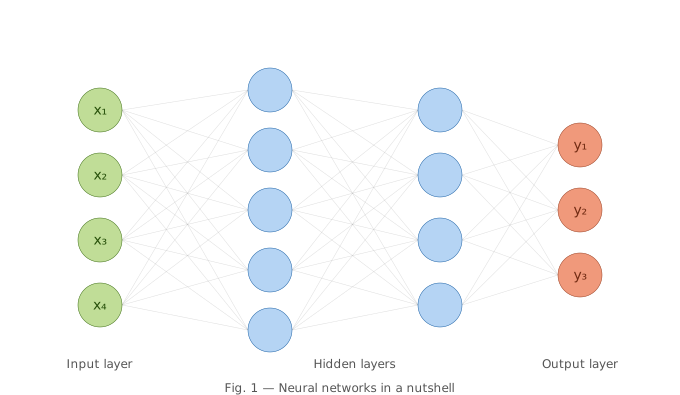
The input layer receives the features, the hidden layers transform them, and the output layer produces the predicted model parameters.
Formal definition of a Multi-Layer Perceptron network (click to expand)
Let $L \in \mathbb{N}$ be the number of layers, and $(N_1, N_2, \dots, N_L) \in \mathbb{N}^L$ the number of neurons in each layer. For $1 \leq l \leq L-1$, we define affine transformations:
$$ a^l: \mathbb{R}^{N_l} \rightarrow \mathbb{R}^{N_{l+1}}, \quad x \mapsto W^{l+1}x + b^{l+1} $$where $W^{l+1} \in \mathbb{R}^{N_{l+1} \times N_l}$ and $b^{l+1} \in \mathbb{R}^{N_{l+1}}$. The network is then the composition:
$$ F := F_{L-1} \circ \dots \circ F_1, \quad \text{with } F_l = \sigma_l \circ a^l $$where $\sigma_l$ is a nonlinear activation function applied component-wise to the output of the affine function $a^l$. For a regression network such as ours, the final layer uses the identity activation.
In our framework, the neural network takes a full implied volatility surface as input and outputs the corresponding model parameters.
The implied volatility surface can be represented as a flattened array, where each element corresponds to a maturity–strike pair defined on a fixed grid. Consequently, we must define a maturity–strike grid on which the learning will be performed. The input dimension of the neural network is therefore:
\[ \text{number of maturities} \times \text{number of strikes}. \]For a new implied volatility surface, it is necessary to interpolate the observed data onto this predefined grid before feeding it into the neural network for prediction.
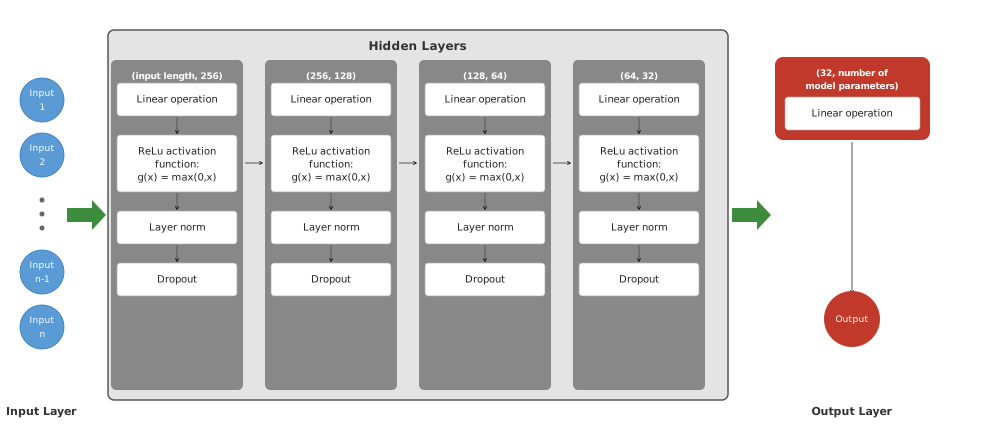
We use a Multi-Layer Perceptron (MLP) architecture composed of four hidden layers, each with a ReLU activation function, layer normalization, and dropout. The ReLU activation function is defined by $x \mapsto \max(0,x)$. Dropout randomly deactivates neurons during training and is intended to reduce overfitting; we use a 1% dropout rate. A larger or deeper network could improve approximation capacity, at the cost of more expensive training and inference. We use:
- He initialization, which is well suited to ReLU-like activation functions.
- Mean Squared Error (MSE) as the loss function on standardized model parameters: $$ D(y, \hat{y}) = ||\hat y - y ||^2_2 $$
Step 1: Construct the learning database
We consider the Heston model as a use case in this section.
$$ \begin{aligned} dX_t &= \sqrt{v_t}X_t\,dW^X_t, \\ dv_t &= \kappa(\theta - v_t)\,dt + \sigma_v \sqrt{v_t}\,dW^v_t, \\ d\langle W^X, W^v\rangle_t &= \rho\,dt \end{aligned} $$where the model parameters are:
- $\kappa$ the speed of mean reversion of variance;
- $\theta$ the long-run variance level;
- $\sigma_v$ the volatility of volatility;
- $\rho$ the correlation between the two Wiener processes $W^X$ and $W^v$;
- $v_0$ the initial variance.
See [LexiFi] for details on our Heston model.
This setting is non-trivial, as the Heston model is known to be non-identifiable: multiple parameter sets may produce similar model outputs. As a result, different parameter configurations may solve the calibration problem equally well. However, the literature suggests that the calibration landscape is locally identifiable, even if it is globally non-injective.
We define a maturity–strike grid composed of 13 maturities ranging from 0.05 to 10 years, and 30 forward moneyness (strike-to-forward ratio) levels uniformly spaced between 0.3 and 5.0. Consequently, the input dimension of the neural network is 390, while the output dimension (corresponding to the Heston parameters) is 5.
To construct the dataset, we collect LexiFi vanilla options market data across thousands of equity underlyings, covering the period from January 2017 to September 2025. We retain only sufficiently liquid underlyings.
For each date and each underlying:
-
We interpolate the observed implied volatility surface onto the predefined maturity–strike grid. The interpolation method is based on the SVI parameterization introduced by Jim Gatheral. The implementation follows the methodology described in [DMM].
-
We calibrate the Heston model to the resulting implied volatility surface using the standard LexiFi calibration framework.
-
Each data point is constructed by concatenating the flattened implied volatility surface (input) with the corresponding calibrated Heston parameters (output).
This process results in a dataset containing several million observations with 395 columns. Processing it is computationally expensive because of its scale and may therefore be performed in batches. This is an offline cost: once the network has been trained, the resulting checkpoint can be reused for many online calibrations.
The network contains 143,493 trainable parameters. Dataset size alone does not guarantee generalization: the observations must also cover a wide range of underlyings, time periods, and market regimes, including stressed conditions. Performance must then be assessed on data excluded from training.
Step 2: Train the neural network
Once the dataset has been constructed, the neural network is trained to minimize the discrepancy between the parameters produced by the reference calibration and those predicted by the network. Training consists of finding the weights and biases that minimize a given loss function. The associated optimization problem can be written as:
\[ \arg \min_{\boldsymbol{\theta}} L(\boldsymbol{\theta}; \mathbf{X}, \mathbf{Y}). \]Here, $\boldsymbol{\theta}$ denotes the parameters of the neural network.
The loss function is defined as:
\[ L(\boldsymbol{\theta}; \mathbf{X}, \mathbf{Y}) = \frac{1}{N} \sum_{i=1}^N D\big(Y_i, \hat{Y}_i(\boldsymbol{\theta}, X_i)\big), \]where $D$ is the MSE metric measuring the discrepancy between reference and predicted standardized parameters. Standardizing the five outputs prevents parameters with larger numerical scales from dominating the loss.
The training of neural networks relies on two fundamental components:
- The backpropagation algorithm, which computes the gradients of the loss function with respect to the network parameters.
- An optimization method (e.g., stochastic gradient descent and its variants), which updates the parameters to minimize the loss.
Together, these components enable the efficient solution of the above optimization problem.
Neural networks' backpropagation and optimization methods (click to expand)
The backpropagation algorithm is designed to compute efficiently the gradients of a loss function $\mathcal{L}$ with respect to all network parameters $\boldsymbol{\theta}$. It is based on a recursive application of the chain rule for derivatives across the different layers of the network. Concretely, at a given layer $\ell$, the input of the layer being $\mathbf{a}^{(\ell-1)}$, its weights and bias being $\mathbf{W}^{(\ell)}$ and $\mathbf{b}^{(\ell)}$ respectively, the layer computes:
$$ \mathbf{z}^{(\ell)} = \mathbf{W}^{(\ell)} \mathbf{a}^{(\ell-1)} + \mathbf{b}^{(\ell)} $$$$ \mathbf{a}^{(\ell)} = \sigma^{(\ell)}(\mathbf{z}^{(\ell)}), \quad \text{ with } \sigma^{(\ell)}\text{ the activation function} $$then the gradients are computed as follows:
$$ \begin{aligned} \frac{\partial \mathcal{L}}{\partial \mathbf{W}^{(\ell)}} &= \frac{\partial \mathcal{L}}{\partial \mathbf{z}^{(\ell)}} \left(\mathbf{a}^{(\ell-1)}\right)^T, \\ \frac{\partial \mathcal{L}}{\partial \mathbf{b}^{(\ell)}} &= \frac{\partial \mathcal{L}}{\partial \mathbf{z}^{(\ell)}}, \\ \frac{\partial \mathcal{L}}{\partial \mathbf{a}^{(\ell-1)}} &= \left(\mathbf{W}^{(\ell)}\right)^T \frac{\partial \mathcal{L}}{\partial \mathbf{z}^{(\ell)}}. \end{aligned} $$These gradients are propagated backwards from the output layer ($\ell = L$) to the input layer ($\ell = 1$), allowing the full computation of parameter updates for gradient-based optimization.
Once gradients are computed, optimization algorithms are used to minimize the loss function in the high-dimensional parameter space. One popular method is Stochastic Gradient Descent (SGD), which calculates gradients using individual data points or mini-batches:
$$ \boldsymbol{\theta}_{t+1} = \boldsymbol{\theta}_t - \eta \nabla_{\boldsymbol{\theta}} \mathcal{L}(\boldsymbol{\theta}_t). $$More advanced methods include adaptive learning rate algorithms such as:
-
AdaGrad: adjusts learning rates using the historical sum of squared gradients:
$$ \boldsymbol{\theta}_{t+1} = \boldsymbol{\theta}_t - \frac{\eta}{\sqrt{G_t + \epsilon}} \odot \mathbf{g}_t, $$where $G_t = \sum_{i=1}^t \mathbf{g}_i \odot \mathbf{g}_i$ and $\mathbf{g}_i = \nabla_{\boldsymbol{\theta}} \mathcal{L}(\boldsymbol{\theta}_i)$.
-
RMSprop: maintains an exponentially decaying average of past squared gradients:
$$ \mathbf{v}_t = \beta \mathbf{v}_{t-1} + (1-\beta) \mathbf{g}_t^2, \quad \boldsymbol{\theta}_{t+1} = \boldsymbol{\theta}_t - \frac{\eta}{\sqrt{\mathbf{v}_t + \epsilon}} \mathbf{g}_t. $$ -
Adam (Adaptive moment estimation): combines momentum and adaptive learning rates
$$ \begin{aligned} \mathbf{m}_t &= \beta_1 \mathbf{m}_{t-1} + (1-\beta_1) \mathbf{g}_t, \\ \mathbf{v}_t &= \beta_2 \mathbf{v}_{t-1} + (1-\beta_2) \mathbf{g}_t^2, \\ \hat{\mathbf{m}}_t &= \frac{\mathbf{m}_t}{1-\beta_1^t}, \quad \hat{\mathbf{v}}_t = \frac{\mathbf{v}_t}{1-\beta_2^t}, \\ \boldsymbol{\theta}_{t+1} &= \boldsymbol{\theta}_t - \frac{\eta}{\sqrt{\hat{\mathbf{v}}_t} + \epsilon} \hat{\mathbf{m}}_t. \end{aligned} $$
These optimization strategies are critical for navigating the often non-convex and high-dimensional landscapes encountered in deep learning applications. We use Adam, which combines momentum with adaptive learning rates and works well for this high-dimensional, non-convex optimization problem.
A complete pass through the training dataset constitutes an epoch. The optimizer updates the network parameters after each mini-batch within an epoch. Additional epochs can improve the fit, but training for too long may lead to overfitting. In our case, the network is trained for 250 epochs.
Step 3: Predict financial model parameters
At this stage, the neural network has learned the relationship, present in the training data, between implied volatility surfaces and the corresponding reference-calibrated model parameters. Its exported checkpoint contains the architecture, weights, biases, output normalization data, and the maturity–strike input grid required by Apropos.
Using this checkpoint, Apropos can efficiently produce an initial parameter prediction for a new input through a sequence of elementary operations implemented natively.
Interpolation of the implied volatility surface
A necessary preliminary step is to transform the observed implied volatility surface into the input format expected by the network. This requires interpolating the surface onto the predefined maturity–strike grid.
The choice of interpolation method directly impacts both the calibration speed and its accuracy. Additional criteria may also be considered when selecting an appropriate method, such as the absence of arbitrage and robustness.
We propose four interpolation schemes:
- Gatheral Stochastic Volatility Inspired (SVI) parameterization: The SVI parameterization has become the market standard because it enforces no static arbitrage across strikes and provides a parsimonious yet flexible representation of the volatility smile.
Details on Gatheral SVI parameterization (click to expand)
For each fixed maturity $T$, we fit the implied volatility smile using Gatheral’s Stochastic Volatility Inspired (SVI) parameterization. It expresses the implied variance as
$$ w(T,x) = \sigma^2(T,K) \, T = a + b\left(\rho(x-m)+\sqrt{(x-m)^2+\sigma^2}\right), $$where $x = \log(K/F(0,T))$ is the log-forward moneyness, $\sigma(T,x)$ the implied volatility at maturity T and strike K, $(a,b,\rho,m,\sigma)$ are the parameters with $a \in \mathbb{R}, b \geq 0,|\rho|<1, m \in \mathbb{R}, \sigma>0$, and the condition $a+b \sigma \sqrt{1-\rho^2} \geq 0$, which ensures that $w(T,x) \geq 0$ for all $x \in \mathbb{R}$. This condition indeed ensures that the minimum of the function $w(T,.)$ is non-negative. Note further that the function $x \mapsto w(T,x)$ is (strictly) convex on the whole real line. Once calibrated to market quotes, this SVI parameterization yields a smooth and arbitrage-free curve $\sigma(T, K)$ for each maturity slice.
Then, to obtain a continuous volatility surface across maturity, we use the method of Andreasen & Huge (2011), described in [AH]. The interpolation operates on call prices, with implied volatilities recovered afterwards by inverting the Black–Scholes formula.
Assuming deterministic interest rates and proportional dividend yields, let $D(0,T)$ be the discount factor, $F(0,T)$ the forward price, and $z=K/F(0,T)$ the forward moneyness. The normalized call price is
$$ c(T,z)=\frac{C(T,zF(0,T))}{D(0,T)F(0,T)}. $$In these coordinates, the Dupire forward equation takes the drift-free form
$$ \frac{\partial c}{\partial T}=\frac{1}{2}\sigma_{\mathrm{loc}}^2(T,z)z^2\frac{\partial^2 c}{\partial z^2}, $$where $\sigma_{\mathrm{loc}}(T,z)$ denotes local volatility evaluated at strike $zF(0,T)$.
For each interval $[T_i,T_{i+1}]$, the Andreasen–Huge scheme calibrates a nonnegative, strike-dependent volatility proxy $\nu_i(z)$ so that a single implicit finite-difference step matches the target call prices at $T_{i+1}$. These targets are obtained from the fitted maturity smiles. The same proxy is used to fill the maturity gap:
$$ \left[1-\frac{1}{2}(T-T_i)\nu_i(z)^2z^2\frac{\partial^2}{\partial z^2}\right]c(T,z)=c(T_i,z), \quad T_i \leq T \leq T_{i+1}. $$The strike derivatives are discretized on a numerical grid, starting from $c(0,z)=(1-z)^+$. The calibrated proxy $\nu_i$ is a coefficient of this one-step scheme; it is distinct from both implied volatility and the local volatility recovered from the resulting continuous-maturity price surface. Finally, the interpolated call prices are converted back to implied volatilities on the network’s input grid.
- Surface SVI (SSVI): performs an SVI-like parameterization for an entire surface at once and ensures absence of arbitrage, based on [GJ].
Details on SSVI parameterization (click to expand)
Let $\varphi$ be a smooth function from $\mathbb{R}_{+}^*$ to $\mathbb{R}_{+}^*$ such that the limit $\lim _{t \rightarrow 0} \theta_t \varphi\left(\theta_t\right)$ exists in $\mathbb{R}$. We refer to SSVI the surface defined by
$$ w\left(k, \theta_t\right)=\frac{\theta_t}{2}\left\{1+\rho \varphi\left(\theta_t\right) k+\sqrt{\left(\varphi\left(\theta_t\right) k+\rho\right)^2+\left(1-\rho^2\right)}\right\} $$The SSVI surface is free of static arbitrage if the following conditions are satisfied:
- $\partial_t \theta_t \geq 0$, for all $t>0$
- $0 \leq \partial_\theta(\theta \varphi(\theta)) \leq \frac{1}{\rho^2}\left(1+\sqrt{1-\rho^2}\right) \varphi(\theta)$, for all $\theta>0$;
- $\theta \varphi(\theta)(1+|\rho|)<4$, for all $\theta>0$;
- $\theta \varphi(\theta)^2(1+|\rho|) \leq 4$, for all $\theta>0$.
We choose as function $\varphi$ the modified power-law parameterization, with $\eta>0$ and $0\leq\gamma\leq\tfrac12$:
$$ \varphi(\theta)=\frac{\eta}{\theta^\gamma(1+\theta)^{1-\gamma}} $$With $|\rho|<1$ and nondecreasing ATM total variance $\theta_t$, this function gives a surface free of static arbitrage provided that $\eta(1+|\rho|) \leq 2$.
- Extended Surface SVI (eSSVI): An extension of SSVI with a parametric form for the leverage parameter. This is motivated by an experiment: the authors of [HM] calibrate SSVI slices on each available maturity so that the only difference with the classical SSVI is that the parameter $\rho$ is not constant. This gives a different value for each slice demonstrating that $\rho$ is not constant, this is particularly noticeable in short maturities.
Details on Parametric eSSVI parameterization (click to expand)
Therefore, the authors formulate the following parameterization $$ w\left(k, \theta_t\right)=\frac{\theta_t}{2}\left\{1+\rho(\theta_t) \varphi\left(\theta_t\right) k+\sqrt{\left(\varphi\left(\theta_t\right) k+\rho(\theta_t)\right)^2+\left(1-\rho(\theta_t)^2\right)}\right\} $$The authors construct a parametric family for $\rho(\theta)$ satisfying sufficient no-calendar-spread conditions up to some maximum maturity. With the modified power-law parameterization of $\varphi$ above, we use
$$ \rho(\theta)=\rho_0+\left(\rho_m-\rho_0\right)\left(\frac{\theta}{\theta_{\max }}\right)^a $$This function is defined up to some maximum maturity corresponding to a total ATM variance $\theta_{max}$. The function is then a monotonous function from $\left(0, \rho_0\right)$ to $\left(\theta_{\text {max }}, \rho_m\right)$ assuming $a \geq 0$, and the second boundary of a reads:
$$ a \leq \begin{cases}\frac{(1-\gamma)\left(1-\rho_m\right)}{\left(1+\theta_{\max }\right)\left(\rho_m-\rho_0\right)} & \text { if } \rho_0<\rho_m \\ \frac{(1-\gamma)\left(1+\rho_m\right)}{\left(1+\theta_{\max }\right)\left(\rho_0-\rho_m\right)} & \text { if } \rho_0>\rho_m\end{cases} $$If $\rho_0=\rho_m$, the correlation is constant and this restriction on $a$ is unnecessary.
For butterfly arbitrage, we impose $\theta\varphi(\theta)(1+|\rho(\theta)|)<4$ and $\theta\varphi(\theta)^2(1+|\rho(\theta)|)\leq4$ at every $0<\theta\leq\theta_{\max}$. Substituting our modified power law gives
$$ \eta \leq \min \left(\frac{4\theta^{\gamma-1}(1+\theta)^{1-\gamma}}{1+|\rho(\theta)|}, \frac{2\theta^{\gamma-1/2}(1+\theta)^{1-\gamma}}{\sqrt{1+|\rho(\theta)|}}\right) $$Since $\rho$ is monotone, a conservative sufficient replacement is therefore
$$ \eta \leq \min \left(\frac{4\theta^{\gamma-1}(1+\theta)^{1-\gamma}}{1+\max \left(\left|\rho_m\right|,\left|\rho_0\right|\right)}, \frac{2\theta^{\gamma-1/2}(1+\theta)^{1-\gamma}}{\sqrt{1+\max \left(\left|\rho_m\right|,\left|\rho_0\right|\right)}}\right), $$- Global eSSVI: a version of eSSVI without any parametric forms on parameters $\varphi$ and $\rho$, based on [MA]
Details on Global eSSVI parameterization (click to expand)
Setting $\psi:=\theta \varphi$, the eSSVI formula in terms of the parameters $(\theta, \rho, \psi)$ becomes
$$ w(k, T)=\frac{1}{2}\left(\theta(T)+\rho(T) \psi(T) k+\sqrt{(\psi(T) k+\theta(T) \rho(T))^2+\theta(T)^2\left(1-\rho(T)^2\right)}\right) $$The Global eSSVI is a model which uses a new global parametrization for a set of consecutive SSVI slices, satisfying the no arbitrage conditions. Given $N$ maturities, the parametrization involves $3 \times N$ parameters.
The new parameters are
$$ \left.\rho_1, \ldots, \rho_N, \theta_1, a_2, \ldots, a_N, c_1, \ldots, c_N \in \right]-1,1\left[^N \times\right] 0, \infty\left[{ }^N \times\right] 0,1\left[^N\right. $$where the $\rho_i$ are the original eSSVI parameters while the $a_i$ and $c_i$ are defined as
$$ \begin{aligned} a_i & =\theta_i-\theta_{i-1} p_i \\ c_i & =\frac{\psi_i-A_{\psi_i}}{C_{\psi_i}-A_{\psi_i}} \end{aligned} $$and
$$ \begin{aligned} p_i &:=\max \left(\frac{1+\rho_{i-1}}{1+\rho_i}, \frac{1-\rho_{i-1}}{1-\rho_i}\right) & \text { if } i>1, \\ f_i &:=\min \left(\frac{4}{1+\left|\rho_i\right|}, \sqrt{\mathfrak{f}\left(\theta_i,\left|\rho_i\right|\right)}\right) & \text { if } i \geq 1, \\ A_{\psi_1} &:=0 & \text { if } i=1, \\ A_{\psi_i} &:=\psi_{i-1} p_i & \text { if } i>1, \\ C_{\psi_1} &:=\min \left(f_1, \frac{f_2}{p_2}, \ldots, \frac{f_N}{\prod_{j=2}^N p_j}\right) & \text { if } i=1, \\ C_{\psi_i} &:=\min \left(\frac{\psi_{i-1}}{\theta_{i-1}} \theta_i, f_i, \frac{f_{i+1}}{p_{i+1}}, \ldots, \frac{f_N}{\prod_{j=i+1}^N p_j}\right) & \text { if } i>1 . \end{aligned} $$we take $\mathfrak{f}\left(\theta,\left|\rho\right|\right) = \frac{4\theta}{1+\left|\rho\right|}$ but other functions could be used as mentioned in [MA].
The eSSVI parameters are sequentially obtained through the ordered relations
$$ \begin{aligned} & \theta_2=\theta_1 p_2+a_2, \quad \ldots, \quad \theta_N=\theta_{N-1} p_N+a_N \\ & \psi_1=c_1\left(C_{\psi_1}-A_{\psi_1}\right)+A_{\psi_1}, \ldots, \psi_N=c_N\left(C_{\psi_N}-A_{\psi_N}\right)+A_{\psi_N} \end{aligned} $$The set of N SSVI slices defined through this scheme is demonstrated to be free of Butterfly and Calendar spread arbitrage. See [MA] for more details.
The calibration
Once the implied volatility surface has been formatted according to the network input, the inference step is straightforward. The network predicts an initial set of financial model parameters based on the relationship learned from the historical reference calibrations.
The prediction is then clipped to the admissible Heston parameter domain and used to define a bounded neighborhood for a local least-squares optimization. This refinement searches for parameters that improve the fit to the current market quotes while retaining the speed benefit of avoiding a broad global search.
In the traditional LexiFi calibration framework, Differential Evolution supplies the global search before local optimization. In the alternative workflow, the neural network replaces that global search with a single MLP forward pass. The inference itself is inexpensive, but the total online calibration time also includes interpolation and local refinement and therefore depends strongly on the selected interpolation technique.
Step 4: Fine-tune the neural network
Will the neural network remain accurate over time? How will it behave under changing market conditions?
To prevent the model from becoming outdated, it must be periodically updated with recent data. Training a pre-trained machine learning model to improve its performance on new data is known as fine-tuning, and it is generally a delicate process.
In our case, the objective is to adapt the network to observed market conditions without erasing previously learned information or drifting too far from its initial state.
-
At each update, recent market data are collected and a new dataset is constructed as in Step 1. The current network is then trained on this new data. However, this training must differ from the initial training (Step 2); otherwise, the network may overfit recent data and forget past information. This phenomenon is known as catastrophic forgetting.
-
To mitigate catastrophic forgetting, we employ techniques that control the deviation between successive states of the network:
- Discriminative fine-tuning: different parts of the network are updated with different learning rates or optimization settings.
- Gradual unfreezing: layers are initially frozen to preserve learned features, then progressively unfrozen during training.
- L2 regularization toward the starting point: a penalty term is added to the loss function to discourage large deviations from the initial parameters.
How to experiment it in LexiFi Apropos ?
At this time, this methodology is available for the Heston model. Its relevance is expected to increase for more complex models, where traditional calibration becomes increasingly time-consuming. Indeed, neural network–based calibration has a nearly constant inference cost, while only the dataset construction scales with model complexity.
For the Heston model, users can choose, as global step for the calibration, between:
- A traditional global optimization method (Differential Evolution).
- The neural network–based approach described above.
When using the neural network, user must specify the neural network representation file and an interpolation method among SVI, SSVI, parametric eSSVI, and global eSSVI.
This approach integrates seamlessly with all applications of the LexiFi solution related to the Heston model. It can be used in any environment and produces highly satisfactory results, allowing clients to achieve significant economies of scale.
Some results
As an initial out-of-sample comparison, we calibrate the Heston model to EURO STOXX 50 data observed on 2026-02-02 (out-of-sample). The table compares the fit obtained with Differential Evolution and with each neural-network interpolation method.
| Calibration method (global step) |
Price RMSE |
Volatility RMSE |
Monte Carlo price RMSE |
Monte Carlo volatility RMSE |
|---|---|---|---|---|
| Benchmark: Differential Evolution | 0.22% | 14.28% | 0.15% | 16.67% |
| Neural network with SVI | 0.25% | 16.14% | 0.10% | 16.42% |
| Neural network with SSVI | 0.23% | 14.17% | 0.12% | 16.64% |
| Neural network with parametric eSSVI | 0.22% | 15.10% | 0.15% | 17.31% |
| Neural network with global eSSVI | 0.28% | 15.75% | 0.12% | 17.74% |
The price RMSE (respectively, volatility RMSE) is defined as the root mean squared error between the observed market prices (respectively, implied volatilities) and the theoretical analytic prices (respectively, implied volatilities) computed using the calibrated model parameters.
Similarly, the Monte Carlo price RMSE (respectively, Monte Carlo volatility RMSE) is the root mean squared error between the observed market prices (respectively, implied volatilities) and the theoretical Monte Carlo prices (respectively, implied volatilities) obtained using the calibrated model parameters.
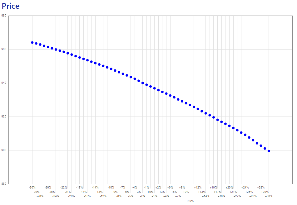
Under normal market conditions, neural network calibration is highly accurate regardless of the interpolation method. Under stressed conditions, however, the choice of interpolation becomes significant. More robust interpolation techniques help maintain high calibration accuracy.
We illustrate this with stressed pricing of a 1-year autocallable product on EURO STOXX 50, with an initial fixing date of 2026-02-12 (out-of-sample). The implied volatility surface is shocked via parallel shifts, and calibration is performed for each scenario to compute the resulting prices.
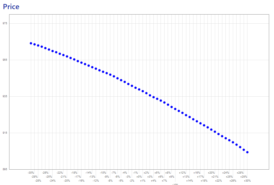 Differential Evolution |
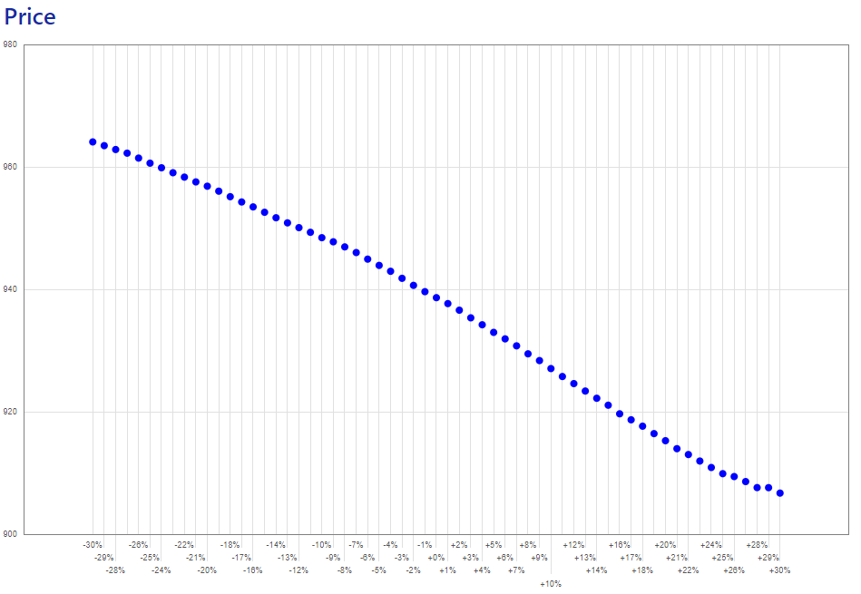 MLP with SSVI |
 MLP with eSSVI |
The choice of interpolation method primarily affects the overall calibration time. Indeed, in the neural network–based approach, the inference step itself is computationally negligible, while the interpolation stage can vary in time complexity depending on the method employed. As a result, the total calibration time is largely driven by the interpolation procedure.
To quantify this effect, we measure the time spent in each calibration step —interpolation, global initialization, and local refinement— in CPU cycles, using a 10-year autocallable product on a basket of the S&P 500, EURO STOXX 50, and Nikkei 225 indices. Timings are collected on a 64 GB RAM desktop equipped with an Intel® Core™ Ultra X7 358H processor (1.90 GHz). The Differential Evolution global step is capped at 2,000 iterations, and the local step is capped at 500 iterations across all methods.
| Calibration method | Interpolation | Global step | Local step | Total (billion CPU cycles) |
Relative to Differential Evolution |
|---|---|---|---|---|---|
| Benchmark: Differential Evolution | 98.06% | 1.94% | 2.42 | 1.00x | |
| Neural network with SVI | 98.28% | 0.02% | 1.70% | 4.54 | 1.87x |
| Neural network with SSVI | 93.35% | 0.08% | 6.57% | 1.10 | 0.46x |
| Neural network with parametric eSSVI | 81.54% | 0.24% | 18.22% | 0.78 | 0.32x |
| Neural network with global eSSVI | 95.29% | 0.05% | 4.66% | 1.98 | 0.82x |
The interpolation, global step, and local step columns report each stage’s share of the total calibration time. In the last column, values below 1.00x indicate a faster calibration than the traditional Differential Evolution framework.
Our experiments show that neural network–based calibration can be more time-consuming than Differential Evolution when using Gatheral’s SVI interpolation. In contrast, when using surface-based interpolation methods (SSVI, eSSVI or global eSSVI), the neural network approach becomes faster overall while maintaining a high level of accuracy. This advantage can be particularly significant in applications requiring a large number of calibrations, such as risk analysis, scenario generation, or portfolio-wide valuations.
Conclusion
We have developed a neural network–based framework for the calibration of financial models, with the goal of achieving both speed and accuracy. The objective was to replicate existing mathematical models with very high fidelity by training machine learning models. Neural networks, as powerful universal function approximators, are well suited to approximating the calibration mapping.
This methodology needs less computational resources and generally less time for calibration than a traditional approach while leading to competitive results.
This methodology integrates naturally into the LexiFi calibration framework and interacts seamlessly with all features and applications related to calibration within the LexiFi solution.
References
[AH] ANDREASEN, Jesper and HUGE, Brian. Volatility Interpolation. Risk, 2011, vol. 24, no 3, p. 76–79. papers.ssrn.com
[DMM] DE MARCO, S. et MARTINI, C. Quasi-explicit calibration of Gatheral’s SVI model. Zeliade White Paper, 2009, p. 1-15. www.zeliade.com
[GJ] GATHERAL, Jim et JACQUIER, Antoine. Arbitrage-free SVI volatility surfaces. Quantitative Finance, 2014, vol. 14, no 1, p. 59-71. //arxiv.org
[HM] HENDRIKS, Sebas et MARTINI, Claude. The extended SSVI volatility surface. Available at SSRN 2971502, 2017. //papers.ssrn.com
[LexiFi] LexiFi model documentation, Heston model, www.lexifi.com
[MA] MINGONE, Arianna. No arbitrage global parametrization for the eSSVI volatility surface. Quantitative Finance, 2022, vol. 22, no 12, p. 2205-2217. //arxiv.org